3 General Principles
This chapter develops a common framework for the modeling of complex systems by using discreteevent simulation. It covers the basic building blocks of all discrete-event simulation models: entities and attributes, activities, and events. In discrete-event simulation, a system is modeled in terms of its state at each point in time; of the entities that pass through the system and the entities that represen system resources; and of the activities and events that cause the system state to change. Discrete-event models are appropriate for those systems for which changes in system state occur only at discrete points in time.
The discussion in this chapter focuses on the discrete-event concepts and methodologies of simulation languages and software (collectively called simulation packages).
This chapter introduces and explains the fundamental concepts and methodologies underlying al discrete-event simulation packages. These concepts and methodologies are not tied to any particular package. Many of the packages use different terminology from that used here, and most have a number of higher-level constructs designed to make modeling simpler and more straightforward for their application domain. For example, this chapter discusses the fundamental abstract concept of an entity, but not covered are more concrete realizations of entities, such as machines, conveyors, and vehicles that are built into some of the packages to facilitate modeling in the manufacturing, materia handling, or other domains
Section 1 covers the general principles and concepts of discrete-event simulation, the even scheduling/time advance algorithm, and the three prevalent world views: event scheduling, process interaction, and activity scanning. Section 2 introduces some of the notions of list processing, one of the more important methodologies used in discrete-event simulation software.
1 Concepts in Discrete-Event Simulation
This chapter deals exclusively with dynamic, stochastic systems (i.e., involving time and containing random elements) that change in a discrete manner. This section expands on these concepts and proposes a framework for the development of a discrete-event model of a system. The major concepts are briefly defined and then illustrated by examples:
System A collection of entities (e.g., people and machines) that interact together over time to accomplish one or more goals.
Model An abstract representation of a system, usually containing structural, logical, or mathematical relationships that describe a system in terms of state, entities and their attributes, sets, processes, events, activities, and delays.
System state A collection of variables that contain all the information necessary to describe the system at any time.
Entity Any object or component in the system that requires explicit representation in the mode (e.g., a server, a customer, a machine).
Attributes The properties of a given entity (e.g., the priority of a waiting customer, the routing of a job through a job shop).
List A collection of (permanently or temporarily) associated entities, ordered in some logica fashion (such as all customers currently in a waiting line, ordered by “first come, first served,” or by priority).
Event An instantaneous occurrence that changes the state of a system (such as an arrival of a new customer).
Event notice A record of an event to occur at the current or some future time, along with any associated data necessary to execute the event; at a minimum, the record includes the even type and the event time.
Event list A list of event notices for future events, ordered by time of occurrence; also known as the future event list (FEL).
Activity A duration of time of specified length (e.g., a service time or interarrival time), which is known when it begins (although it may be defined in terms of a statistical distribution).
Delay A duration of time of unspecified indefinite length, which is not known until it ends (e.g., a customer’s delay in a last-in–first-out waiting line which, when it begins, depends on future arrivals).
Clock A variable representing simulated time, called CLOCK in the examples to follow.
Different simulation packages use different terminology for the same or similar concepts—for example, lists are sometimes called sets, queues, or chains. Sets or lists are used to hold both entities and event notices. The entities on a list are always ordered by some rule, such as first-in–first-out or last-in–first-out, or are ranked by some entity attribute, such as priority or due date. The future event list is always ranked by the event time recorded in the event notice. Section 2 discusses a number of methods for handling lists and introduces some of the methodologies for efficient processing o ordered sets or lists.
An activity typically represents a service time, an interarrival time, or any other processing time whose duration has been characterized and defined by the modeler. An activity’s duration may be specified in a number of ways:
a. Deterministic—for example, always exactly 5 minutes;
b. Statistical—for example, as a random draw from the set 2, 5, 7 with equal probabilities;
c. A function depending on system variables and/or entity attributes—for example, loading time for an iron ore ship as a function of the ship’s allowed cargo weight and the loading rate in tons per hour.
However it is characterized, the duration of an activity is computable from its specification at the instant it begins. Its duration is not affected by the occurrence of other events (unless, as is allowed by some simulation packages, the model contains logic to cancel or postpone an activity in progress). To keep track of activities and their expected completion time, at the simulated instant that an activity duration begins, an event notice is created having an event time equal to the activity’s completion time. For example, if the current simulated time is CLOCK 100 minutes and an inspection time of exactly 5 minutes is just beginning, then an event notice is created that specifies the type of even (an end-of-inspection event), and the event time (1005 105 minutes).
In contrast to an activity, a delay’s duration is not specified by the modeler ahead of time, bu rather is determined by system conditions. Quite often, a delay’s duration is measured and is one of the desired outputs of a model run. Typically, a delay ends when some set of logical conditions becomes true or one or more other events occur. For example, a customer’s delay in a waiting line may be dependent on the number and duration of service of other customers ahead in line as well as the availability of servers and equipment.
A delay is sometimes called a conditional wait, an activity an unconditional wait. The completion of an activity is an event, often called a primary event, that is managed by placing an event notice on the FEL. In contrast, delays are managed by placing the associated entity on another list, perhaps representing a waiting line, until such time as system conditions permit the processing of the entity. The completion of a delay is sometimes called a conditional or secondary event, but such events are not represented by event notices, nor do they appear on the FEL.
The systems considered here are dynamic, that is, changing over time. Therefore, system state, entity attributes and the number of active entities, the contents of sets, and the activities and delays
currently in progress are all functions of time and are constantly changing over time. Time itself is represented by a variable called CLOCK.
Consider the Able–Baker call center system of Example 6 from the Simulation Examples in a Spreadsheet chapter. A discrete-event model has the following components:
System state , the number of callers waiting to be served at time ;, 0 or 1 to indicate Able as being idle or busy at time ;, 0 or 1 to indicate Baker as being idle or busy at time .
Entities Neither the callers nor the servers need to be explicitly represented, except in terms of the state variables, unless certain caller averages are desired (compare Examples 4 and 5).
Events Arrival event; Service completion by Able; Service completion by Baker.
Activities Interarrival time, defined in Table 12 from the Simulation Examples in a Spreadsheet chapter; Service time by Able, defined in Table 13 from the Simulation Examples in a Spreadsheet chapter; Service time by Baker, defined in Table 14 from the Simulation Examples in a Spreadsheet chapter.
Delay A caller’s wait in queue until Able or Baker becomes free.
The definition of the model components provides a static description of the model. In addition, a description of the dynamic relationships and interactions between the components is also needed. Some questions that need answers include:
How does each event affect system state, entity attributes, and set contents?
How are activities defined (i.e., deterministic, probabilistic, or some other mathematical equation)? What event marks the beginning or end of each activity? Can the activity begin regardless of system state, or is its beginning conditioned on the system being in a certain state? (For example, a machining “activity” cannot begin unless the machine is idle, not broken, and not in maintenance.)
Which events trigger the beginning (and end) of each type of delay? Under what conditions does a delay begin or end?
What is the system state at time 0? What events should be generated at time 0 to “prime” the model—that is, to get the simulation started?
A discrete-event simulation is the modeling over time of a system all of whose state changes occur at discrete points in time—those points when an event occurs. A discrete-event simulation (hereafter called a simulation) proceeds by producing a sequence of system snapshots (or system images) that represent the evolution of the system through time. A given snapshot at a given time (CLOCK t) includes not only the system state at time t, but also a list (the FEL) of all activities currently in progress and when each such activity will end, the status of all entities and current membership of all sets, plus the current values of cumulative statistics and counters that will be used to calculate summary statistics at the end of the simulation. A prototype system snapshot is shown in Figure 1. (Not all models will contain every element exhibited in Figure 1. Further illustrations are provided in the examples in this chapter.)
1.1 The Event Scheduling/Time Advance Algorithm
The mechanism for advancing simulation time and guaranteeing that all events occur in correc chronological order is based on the future event list (FEL). This list contains all event notices for events that have been scheduled to occur at a future time. Scheduling a future event means that, at the instant an activity begins, its duration is computed or drawn as a sample from a statistical distribution; and that the end-activity event, together with its event time, is placed on the future event list. In the real world, most future events are not scheduled but merely happen—such as random breakdowns or random arrivals. In the model, such random events are represented by the end of some activity, which in turn is represented by a statistical distribution
At any given time t, the FEL contains all previously scheduled future events and their associated event times (called in Figure 1). The FEL is ordered by event time, meaning that the events are arranged chronologically—that is, the event times satisfy
Time t is the value of CLOCK, the current value of simulated time. The event associated with time is called the imminent event; that is, it is the next event that will occur. After the system snapshot at simulation time CLOCK t has been updated, the CLOCK is advanced to simulation time , the imminent event notice is removed from the FEL, and the event is executed. Execution of the imminent event means that a new system snapshot for time is created, one based on the old snapshot at time t and the nature of the imminent event. At time , new future
| CLOCK | System state | Entities and attributes | Set 1 | Set 2 | … | Future event list (FEL) | Cumulative statistics and counters |
|---|---|---|---|---|---|---|---|
| t | (x,y,z,…) | (3,t1)- Type 3 event to occur at time t1(1,t2)- Type 1 event to occur at time t2. . . . . . . . . . . . . . . . . . . . . . . . . . . . . . . . . . . . . . . . . . . . . . . . . . . . . . . . . . . . . . . . . . . . . . . . . . . . . . . . . . . . . . . . . . . . . . . . . . . . . | . . . . . . . . . . . . . . . . . . . . . . . . . . . . . . . . . . . . . . . . . . . . . . . . . . . . . . . . . . . . . . . . . . . . . . . . . . . . . . . . . . . . . . . . . . . . . . . . . . . |
Figure 1 Prototype system snapshot at simulation time t.
events may or might not be generated, but if any are, they are scheduled by creating event notices and putting them into their proper position on the FEL. After the new system snapshot for time has been updated, the clock is advanced to the time of the new imminent event and that event is executed. This process repeats until the simulation is over. The sequence of actions that a simulator (or simulation language) must perform to advance the clock and build a new system snapshot is called the event-scheduling/time-advance algorithm, whose steps are listed in Figure 2 (and explained thereafter).
The length and contents ofthe FEL are constantly changing as the simulation progresses, and thus its efficient management in a simulation software package will have a major impact on the model’s computer runtime. The management of a list is called list processing. The major list processing operations performed on a FEL are removal of the imminent event, addition of a new event to the list, and occasionally removal of some event (called cancellation of an event). As the imminent event is usually at the top of the list, its removal is as efficient as possible. Addition of a new event (and cancellation of an old event) requires a search of the list. The efficiency of this search depends on the logical organization of the list and on how the search is conducted. In addition to the FEL, al the sets in a model are maintained in some logical order, and the operations of addition and remova of entities from the set also require efficient list-processing techniques. A brief introduction to lis processing in simulation is given in Section 2.
The removal and addition of events from the FEL is illustrated in Figure 2. Event 3 with event time represents, say, a service completion event at server 3. Since it is the imminent event at time t, it is removed from the FEL in Step 1 (Figure 2) of the event-scheduling/time-advance algorithm. When event 4 (say, an arrival event) with event time is generated at Step 4, one possible way to determine its correct position on the FEL is to conduct a top-down search:
(In Figure 2, it was assumed that was between and ) Another way is to conduct a bottom-up search. The least efficient way to maintain the FEL is to leave it as an unordered list (additions placed arbitrarily at the top or bottom), which would require at Step 1 of Figure 2 a complete search of the list for the imminent event before each clock advance. (The imminent event is the event on the FEL with the lowest event time.)
The system snapshot at time 0 is defined by the initial conditions and the generation of the so-called exogenous events. The specified initial conditions define the system state at time 0. For example, in Figure , then the state (5, 1, 6) might represent the initial number of customers at three different points in the system. An exogenous event is a happening “outside the system” tha impinges on the system. An important example is an arrival to a queueing system. At time 0, the firs arrival event is generated and is scheduled on the FEL (meaning that its event notice is placed on the FEL). The interarrival time is an example of an activity. When the clock eventually is advanced to the time of this first arrival, a second arrival event is generated. First, an interarrival time, call it , is
Old system snapshot at time t
| CLOCK | System state | Future event list | ||
|---|---|---|---|---|
| (5, 1, 6) |
Event-scheduling/time-advance algorithm
Step 1. Remove the event notice for the imminent event (event 3, time from FEL.
Step 2. Advance CLOCK to imminent event time (i.e., advance CLOCK from t to t ).
Step 3. Execute imminent event: update system state, change entity attributes, and set membership as needed.
Step 4. Generate future events (if necessary) and place their event notices on FEL, ranked by event time. (Example: Event 4 to occur at time t∗, where Step 5. Update cumulative statistics and counters.
New system snapshot at time | CLOCK | System state || Future event list || | — | — | — | — | — | || (5, 1, 5) | || |
Figure 2 Advancing simulation time and updating system image.
generated; it is added to the current time, the resulting (future) event time, is used to position the new arrival event notice on the FEL. This method of generating an external arrival stream is called bootstrapping; it provides one example of how future events are generated in Step 4 of the event-scheduling/time-advance algorithm. Bootstrapping is illustrated in Figure 3.
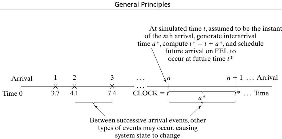 Figure 3 Generation of an external arrival stream by bootstrapping.
The first three interarrival times generated are 3.7, 0.4, and 3.3 time units. The end of an interarriva interval is an example of a primary event.
A second example of how future events are generated (Step 4 of Figure 2) is provided by a service completion event in a queueing simulation. When one customer completes service, at current time if the next customer is present, then a new service time,, will be generated for the next customer. The next service completion event will be scheduled to occur at future time , by placing onto the FEL a new event notice, of type service completion, with event time t∗. In addition, a service-completion event will be generated and scheduled at the time of an arrival event provided that, upon arrival, there is at least one idle server in the server group. A service time is an example of an activity. Beginning service is a conditional event, because its occurrence is triggered only on the condition that a customer be present and a server be free. Service completion is an example of a primary event. Note that a conditional event, such as beginning service, is triggered by a primary event’s occurring and by certain conditions prevailing in the system. Only primary events appear on the FEL.
A third important example is the alternate generation of runtimes and downtimes for a machine subject to breakdowns. At time 0, the first runtime will be generated, and an end-of-runtime even will be scheduled. Whenever an end-of-runtime event occurs, a downtime will be generated, and an end-of-downtime event will be scheduled on the FEL. When the CLOCK is eventually advanced to the time of this end-of-downtime event, a runtime is generated, and an end-of-runtime event is scheduled on the FEL. In this way, runtimes and downtimes continually alternate throughout the simulation. A runtime and a downtime are examples of activities, and end of runtime and end of downtime are primary events.
Every simulation must have a stopping event, here called E, which defines how long the simulation will run. There are generally two ways to stop a simulation:
At time 0, schedule a stop simulation event at a specified future time . Thus, before simulating, it is known that the simulation will run over the time interval . Example: Simulate a job shop for hours.
Run length is determined by the simulation itself. Generally, is the time of occurrence of some specified event E. Examples: could be the time of the 100th service completion
at a certain service center. could be the time of breakdown of a complex system. could be the time of disengagement or total kill (whichever occurs first) in a combat simulation. could be the time at which a distribution center ships the last carton in a day’s orders.
In case is not known ahead of time. Indeed, it could be one of the statistics of primary interest to be produced by the simulation.
1.2 World Views
When using a simulation package or even when doing a manual simulation, a modeler adopts a world view or orientation for developing a model. The most prevalent world views are the eventscheduling world view, as discussed in the previous section, the process-interaction world view, and the activity-scanning world view. Even if a particular package does not directly support one or more of the world views, understanding the different approaches could suggest alternative ways to mode a given system.
To summarize the previous discussion, when using the event-scheduling approach, a simulation analyst concentrates on events and their effect on system state. This world view will be illustrated by the manual simulations of Section 1.3.
When using a package that supports the process-interaction approach, a simulation analyst thinks in terms of processes. The analyst defines the simulation model in terms of entities or objects and their life cycle as they flow through the system, demanding resources and queueing to wait for resources. More precisely, a process is the life cycle of one entity. This life cycle consists of various events and activities. Some activities might require the use of one or more resources whose capacities are limited. These and other constraints cause processes to interact, the simplest example being an entity forced to wait in a queue (on a list) because the resource it needs is busy with another entity. The process-interaction approach is popular because it has intuitive appeal and because the simulation packages that implement it allow an analyst to describe the process flow in terms of high-level block or network constructs, while the interaction among processes is handled automatically.
In more precise terms, a process is a time-sequenced list of events, activities, and delays, including demands for resources, that define the life cycle of one entity as it moves through a system. An example of a “customer process” is shown in Figure 4. In this figure, we see the interaction between two customer processes as customer n 1 is delayed until the previous customer’s “end service event” occurs. Usually, many processes are active simultaneously in a model, and the interaction among processes could be quite complex.
Underlying the implementation of the process interaction approach in a simulation package, bu usually hidden from a modeler’s view, events are being scheduled on a future event list and entities are being placed onto lists whenever they face delays, causing one process to temporarily suspend its execution while other processes proceed. It is important that the modeler have a basic understanding of the concepts and, for the simulation package being used, a detailed understanding of the built-in but hidden rules of operation. Schriber and Brunner [2003] provide understanding in this area.
Both the event-scheduling and the process-interaction approach use a variable time advance— that is, when all events and system state changes have occurred at one instant of simulated time, the simulation clock is advanced to the time of the next imminent event on the FEL. The activity-scanning approach, in contrast, uses a fixed time increment and a rule-based approach to decide whether any activities can begin at each point in simulated time.
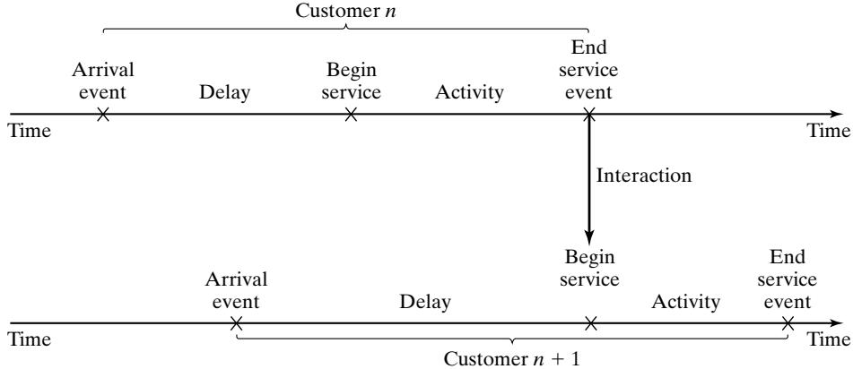 Figure 4 Two interacting customer processes in a single-server queue.
With the activity-scanning approach, a modeler concentrates on the activities of a model and those conditions, simple or complex, that allow an activity to begin. At each clock advance, the conditions for each activity are checked, and, if the conditions are true, then the corresponding activity begins. Proponents claim that the activity-scanning approach is simple in concept and leads to modular models that are more easily maintained, understood, and modified by other analysts a later times. They admit, however, that the repeated scanning to discover whether an activity can begin results in slow runtime on computers. Thus, the pure activity-scanning approach has been modified (and made conceptually somewhat more complex) by what is called the three-phase approach, which combines some of the features of event scheduling with activity scanning to allow for variable time advance and the avoidance of scanning when it is not necessary, but keeps the main advantages o the activity-scanning approach.
In the three-phase approach, events are considered to be activities of duration zero time units. With this definition, activities are divided into two categories, which are called B and C.
B activities activities bound to occur; all primary events and unconditional activities.
C activities activities or events that are conditional upon certain conditions being true.
The B-type activities and events can be scheduled ahead of time, just as in the event-scheduling approach. This allows variable time advance. The FEL contains only B-type events. Scanning to learn whether any C-type activities can begin or C-type events occur happens only at the end of each time advance, after all B-type events have been completed. In summary, with the three-phase approach, the simulation proceeds with repeated execution of the 3 phases until it is completed:
Phase A Remove the imminent event from the FEL and advance the clock to its event time. Remove from the FEL any other events that have the same event time.
Phase B Execute all B-type events that were removed from the FEL. (This could free a number of resources or otherwise change system state.)
Phase C Scan the conditions that trigger each C-type activity and activate any whose conditions are met. Rescan until no additional C-type activities can begin and no events occur.
The three-phase approach improves the execution efficiency of the activity-scanning method. In addition, proponents claim that the activity-scanning and three-phase approaches are particularly good at handling complex resource problems in which various combinations of resources are needed to accomplish different tasks. These approaches guarantee that all resources being freed at a given simulated time will be freed before any available resources are reallocated to new tasks.
Example 2: Call Center, Back Again
For the Call Center in Example 1, ifwe were to adopt the three-phase approach to the activity-scanning world view, the conditions for beginning each activity in Phase C would be as follows:
| Activity | Condition |
|---|---|
| Service time by Able | A caller is in queue and Able is idle |
| Service time by Baker | A caller is in queue, Baker is idle and Able is busy |
Ifit were to take the process-interaction world view, we would view the model from the viewpoint of a caller and its “life cycle.” Considering a life cycle as beginning upon arrival, a customer process is pictured in Figure 4.
In summary, the process-interaction approach has been adopted by the simulation packages most popular in the USA. On the other hand, a number of activity-scanning packages are popular in the UK and Europe. Some of the packages allow portions of a model to be event-scheduling-based, if tha orientation is convenient, mixed with the process-interaction approach. Finally, some of the packages are based on a flow chart, block diagram, or network structure, which upon closer examination turns out to be a specific implementation of the process-interaction concept.
1.3 Manual Simulation Using Event Scheduling
In the conducting ofan event-scheduling simulation, a simulation table is used to record the successive system snapshots as time advances.
Example 3: Single-Channel Queue
Consider the grocery store with one checkout counter that is simulated in Example 5 from the Simulation Examples in a Spreadsheet chapter by an ad hoc method. The system consists of those customers in the waiting line plus the one (if any) checking out. A stopping time of 60 minutes is set for this example. The model has the following components:
System state (LQ(t), LS(t)), where LQ(t) is the number of customers in the waiting line, and LS(t) is the number being served (0 or 1) at time t.
Entities The server and customers are not explicitly modeled, except in terms of the state variables.
Events
Arrival (A);
Departure (D);
Stopping event (E), scheduled to occur at time 60.
Event notices
(A, t), representing an arrival event to occur at future time t;
(D, t), representing a customer departure at future time t;
(E, 60), representing the simulation stop event at future time 60.
Activities
Interarrival time, defined in Table 9 from the Simulation Examples in a Spreadsheet chapter; Service time, defined in Table 10 from the Simulation Examples in a Spreadsheet chapter.
Delay Customer time spent in waiting line.
The event notices are written as (event type, event time). In this model, the FEL will always contain either two or three event notices. The effect of the arrival and departure events is shown in detail in Figures 5 and 6.
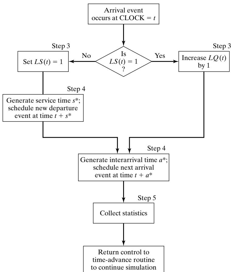 Figure 5 Execution of the arrival event.
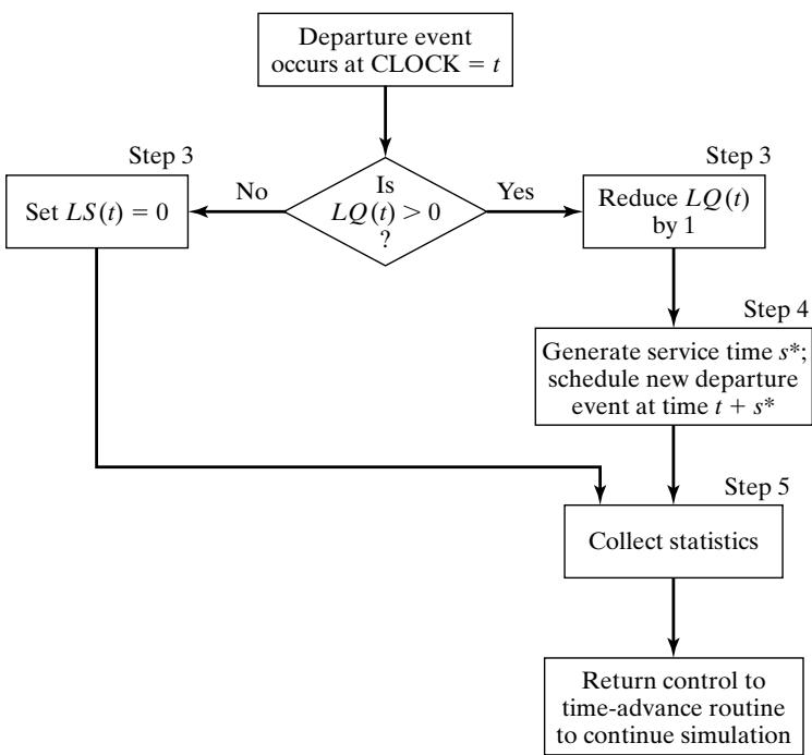 Figure 6 Execution of the departure event.
The simulation table for the checkout counter is given in Table 1. The reader should cover all system snapshots except one, starting with the first, and attempt to construct the next snapshot from the previous one and the event logic in Figures 5 and 6.
| Interarrival Times | 1 | 1 | 6 | 3 | 7 | 5 | 2 | 4 | 1··· |
|---|---|---|---|---|---|---|---|---|---|
| Service Times | 4 | 2 | 5 | 4 | 1 | 5 | 4 | 1 | 4··· |
Initial conditions are that the first customer arrive at time 0 and begin service. This is reflected in Table 1 by the system snapshot at time zero , with , and both a departure event and arrival event on the FEL. Also, the simulation is scheduled to stop at time 60. Only two statistics, server utilization and maximum queue length, will be collected. Server utilization is defined by total server busy time (B) divided by total time ). Total busy time, B, and maximum queue length, MQ, will be accumulated as the simulation progresses. A column headed “Comments” is included to aid the reader and are the generated interarrival and service times, respectively).
As soon as the system snapshot at time CLOCK 0 is complete, the simulation begins. At time 0, the imminent event is . The CLOCK is advanced to time 1, and is removed from the FEL. Because for , the server was busy for 1 minute), the cumulative busy time is increased from to . By the event logic in Figure 6, set (the
Table 1 Simulation Table for Checkout Counter
| CLOCK | System state | Future event list | Comment | Cumulative statistics | ||
|---|---|---|---|---|---|---|
| B | MQ | |||||
| 0 | 0 | 1 | (A, 1) (D, 4) (E, 60) | First A occurs Schedule next A Schedule first D | 0 | 0 |
| 1 | 1 | 1 | (A, 2) (D, 4) (E, 60) | Second A occurs: (A, 1) Schedule next A(Customer delayed) | 1 | 1 |
| 2 | 2 | 1 | (D, 4) (A, 8) (E, 60) | Third A occurs: (A, 2) Schedule next A(Two customers delayed) | 2 | 2 |
| 4 | 1 | 1 | (D, 6) (A, 8) (E, 60) | First D occurs: (D, 4) Schedule next D(Customer delayed) | 4 | 2 |
| 6 | 0 | 1 | (A, 8) (D, 11) (E, 60) | Second D occurs: (D, 6) Schedule next D | 6 | 2 |
| 8 | 1 | 1 | (D, 11) (A, 11) (E, 60) | Fourth A occurs: (A, 8) Schedule next A(Customer delayed) | 8 | 2 |
| 11 | 1 | 1 | (D, 15) (A, 18) (E, 60) | Fifth A occurs: (A, 11) Schedule next AThird D occurs: (D, 11) Schedule next D(Customer delayed) | 11 | 2 |
| 15 | 0 | 1 | (D, 16) (A, 18) (E, 60) | Fourth D occurs: (D, 15) Schedule next D | 15 | 2 |
| 16 | 0 | 0 | (A, 18) (E, 60) | Fifth D occurs: (D, 16) | 16 | 2 |
| 18 | 0 | 1 | (D, 23) (A, 23) (E, 60) | Sixth A occurs Schedule next A Schedule next D | 16 | 2 |
| 23 | 0 | 1 | (A, 25) (D, 27) (E, 60) | Seventh A occurs: (A, 23) Schedule next ArrivalSixth D occurs: (D, 23) | 21 | 2 |
server becomes busy). The FEL is left with three future events, (A, 2), (D, 4), and (E, 60). The simulation CLOCK is next advanced to time 2, and an arrival event is executed. The interpretation of the remainder of Table 1 is left to the reader.
The simulation in Table 1 covers the time interval [0,23]. At simulated time 23, the system empties, but the next arrival also occurs at time 23. The server was busy for 21 of the 23 time units simulated, and the maximum queue length was two. This simulation is, of course, too short to draw any reliable conclusions. Note that the simulation table gives the system state at all times, not jus the listed times. For example, from time 11 to time 15, there is one customer in service and one in the waiting line.
When an event-scheduling algorithm is implemented in simulation software, the software maintains just one set of system states and other attribute values, that is, just one snapshot (the curren one or partially updated one). With the idea of implementing event scheduling in Java or some other general-purpose language, the following rule should be followed. A new snapshot can be derived only from the previous snapshot, newly generated random variables, and the event logic (Figures 5 and 6). Past snapshots should be ignored for advancing of the clock. The current snapshot mus contain all information necessary to continue the simulation.
Example 4: The Checkout-Counter Simulation, Continued
Suppose that, in the simulation of the checkout counter in Example 3, the simulation analyst desires to estimate mean response time and mean proportion of customers who spend 5 or more minutes in the system. A response time is the length of time a customer spends in the system. In order to estimate these customer averages, it is necessary to expand the model in Example 3 to represent the individual customers explicitly. In addition, to be able to compute an individual customer’s response time when that customer departs, it will be necessary to know that customer’s arrival time. Therefore, a customer entity with arrival time as an attribute will be added to the list of model components in Example 3. These customer entities will be stored in a list to be called “CHECKOUT LINE”; they will be called C1, C2, C3, . . . Finally, the event notices on the FEL will be expanded to indicate which customer is affected. For example, (D,4,C1) means that customer C1 will depart at time 4. The additional model components are the following:
Entities
(Ci, t), representing customer Ci who arrived at time t.
Event notices
(A, t, Ci), the arrival of customer Ci at future time t;
(D, t, Cj), the departure of customer Cj at future time t,
Set
“CHECKOUT LINE,” the set of all customers currently at the checkout counter (being served or waiting to be served), ordered by time of arrival
Three new cumulative statistics will be collected: S, the sum of customer response times for al customers who have departed by the current time; F, the total number of customers who spend 5 or more minutes at the checkout counter; and , the total number of departures up to the curren simulation time. These three cumulative statistics will be updated whenever the departure even occurs; the logic for collecting these statistics would be incorporated into Step 5 of the departure event in Figure 6.
Table 2 Simulation Table for Example 4
| CLOCK | System state | CHECKOUT LINE | Future event list | Cumulative statistics | |||
|---|---|---|---|---|---|---|---|
| S | F | ||||||
| 0 | 0 | 1 | (C1,0) | (A,1,C2) (D,4,C1) (E,60) | 0 | 0 | 0 |
| 1 | 1 | 1 | (C1,0) (C2,1) | (A,2,C3) (D,4,C1) (E,60) | 0 | 0 | 0 |
| 2 | 2 | 1 | (C1,0) (C2,1) (C3,2) | (D,4,C1) (A,8,C4) (E,60) | 0 | 0 | 0 |
| 4 | 1 | 1 | (C2,1) (C3,2) | (D,6,C2) (A,8,C4) (E,60) | 4 | 1 | 0 |
| 6 | 0 | 1 | (C3,2) | (A,8,C4) (D,11,C3) (E,60) | 9 | 2 | 1 |
| 8 | 1 | 1 | (C3,2) (C4,8) | (D,11,C3) (A,11,C5) (E,60) | 9 | 2 | 1 |
| 11 | 1 | 1 | (C4,8) (C5,11) | (D,15,C4) (A,18,C6) (E,60) | 18 | 3 | 2 |
| 15 | 0 | 1 | (C5,11) | (D,16,C5) (A,18,C6) (E,60) | 25 | 4 | 3 |
| 16 | 0 | 0 | (A,18,C6) (E,60) | 30 | 5 | 4 | |
| 18 | 0 | 1 | (C6,18) | (D,23,C6) (A,23,C7) (E,60) | 30 | 5 | 4 |
| 23 | 0 | 1 | (C7,23) | (A,25,C8) (D,27,C7) (E,60) | 35 | 6 | 5 |
The simulation table for Example 4 is shown in Table 2. The same data for interarrival and service times will be used again; so Table 2 essentially repeats Table 1, except that the new components are included (and the comment column has been deleted). These new components are needed for the computation of the cumulative statistics S, F, and . For example, at time 4, a departure event occurs for customer C1. The customer entity C1 is removed from the list called “CHECKOUT LINE”; the attribute “time of arrival” is noted to be 0, so the response time for this customer was 4 minutes. Hence, S is incremented by 4 minutes. is incremented by one customer, but F is not incremented, for the time in system was less than five minutes. Similarly, at time 23, when the departure even (D, 23, C6) is being executed, the response time for customer C6 is computed by
Then S is incremented by 5 minutes, and F and by one customer.
For a simulation run length of 23 minutes, the average response time was minutes, and the observed proportion of customers who spent 5 or more minutes in the system was . Again, this simulation was far too short to regard these estimates as having any degree of accuracy. The purpose of Example 4, however, was to illustrate the notion that, in many simulation models, the information desired from the simulation (such as the statistics and to some extent dictates the structure of the model.
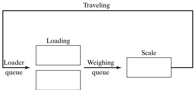 Figure 7 Dump truck problem.
Example 5: The Dump-Truck Problem
Six dump trucks are used to haul coal from the entrance of a small mine to the railroad. Figure 7 provides a schematic of the dump-truck operation. Each truck is loaded by one of two loaders. After a loading, the truck immediately moves to the scale, to be weighed as soon as possible. Both the loaders and the scale have a first-come–first-served waiting line (or queue) for trucks. Travel time from a loader to the scale is considered negligible. After being weighed, a truck begins a travel time (during which time the truck unloads) and then afterward returns to the loader queue.
The distributions of loading time, weighing time, and travel time are given in Tables 3, 4, and 5, respectively. These activity times are generated in exactly the same manner as service times in Section 1.5, Example 2 from the Simulation Examples in a Spreadsheet chapter, using the cumulative probabilities to divide the unit interval into subintervals whose lengths correspond to the probabilities of each individual value. Random numbers come from Table A.1 in the Appendix or one of Excel’s random number generators. A random number is drawn and the interval it falls into determines the next random activity time
The purpose of the simulation is to estimate the loader and scale utilizations (percentage of time busy). The model has the following components:
System state
[LQ(t), L(t), WQ(t), W(t)], where
LQ(t) number of trucks in loader queue;
L(t) number of trucks (0, 1, or 2) being loaded
WQ(t) = number of trucks in weigh queue;
W(t) number of trucks (0 or 1) being weighed, all at simulation time t.
Entities
The six dump trucks (DT1, . . . , DT6).
Event notices
(ALQ, t, DTi), DTi arrives at loader queue (ALQ) at time t;
(EL, t, DTi), DTi ends loading (EL) at time t;
(EW, t, DTi), DTi ends weighing (EW) at time t.
Table 3 Distribution of Loading Time for the Dump Trucks
| Loading Time | Probability | Cumulative Probability | Random Number Interval |
|---|---|---|---|
| 5 | 0.30 | 0.30 | |
| 10 | 0.50 | 0.80 | |
| 15 | 0.20 | 1.00 |
Table 4 Distribution of Weighing Time for the Dump Trucks
| Weighing Time | Probability | Cumulative Probability | Random Number Interval |
|---|---|---|---|
| 12 | 0.70 | 0.70 | |
| 16 | 0.30 | 1.00 |
Table 5 Distribution of Travel Time for the Dump Trucks
| Travel Time | Probability | Cumulative Probability | Random Number Interval |
|---|---|---|---|
| 40 | 0.40 | 0.40 | |
| 60 | 0.30 | 0.70 | |
| 80 | 0.20 | 0.90 | |
| 100 | 0.10 | 1.00 |
Lists
Loader queue, all trucks waiting to begin loading, ordered on a first-come–first-served basis;
Weigh queue, all trucks waiting to be weighed, ordered on a first-come–first-served basis.
Activities
Loading time, weighing time, and travel time.
Delays
Delay at loader queue, and delay at scale.
The simulation table is given in Table 6. To initialize the table’s first row, we assume that, at time 0, five trucks are at the loaders and one is at the scale. For simplicity, we take the (randomly generated) activity times from the following list as needed:
| Loading Time | 10 | 5 | 5 | 10 | 15 | 10 | 10 |
|---|---|---|---|---|---|---|---|
| Weighing Time | 12 | 12 | 12 | 16 | 12 | 16 | |
| Travel Time | 60 | 100 | 40 | 40 | 80 |
When an end-loading (EL) event occurs, say, for dump truck j at time t, other events might be triggered. If the scale is idle , dump truck j begins weighing and an end-weighing even (EW) is scheduled on the FEL; otherwise, dump truck j joins the weigh queue. If, at this time, there is another truck waiting for a loader, it will be removed from the loader queue and will begin loading by the scheduling of an end-loading event (EL) on the FEL. Both this logic for the occurrence of the end-loading event and the appropriate logic for the other two events, should be incorporated into an event diagram, as in Figures 5 and 6 of Example 3. The construction of these event-logic diagrams is left as an exercise for the reader (Exercise 2).
As an aid to the reader, in Table 6, whenever a new event is scheduled, its event time is written as “t (activity time).” For example, at time 0, the imminent event is an EL event with event time 5. The clock is advanced to time , dump truck 3 joins the weigh queue (because the scale is occupied), and dump truck 4 begins to load. Thus, an EL event is scheduled for truck 4 at future time 10, computed by (present time) (loading time) In order to estimate the loader and scale utilizations, two cumulative statistics are maintained:
B total busy time of both loaders from time 0 to time t
Both loaders are busy from time 0 to time , so at time t 20—but, from time 20 to time 24, only one loader is busy; thus, increases by only 4 minutes over the time interval [20, 24]. Similarly, from time 25 to time 36, both loaders are idle , so does not change. For the relatively short simulation in Table 6, the utilizations are estimated as follows:
These estimates cannot be regarded as accurate estimates of the long-run “steady-state” utilizations of the loader and scale; a considerably longer simulation would be needed to reduce the effect of the assumed conditions at time 0 (five of the six trucks at the loaders) and to realize accurate estimates. On the other hand, if the analyst were interested in the so-called transient behavior of the system over a short period of time (say 1 or 2 hours), given the specified initial conditions, then the results in Table 6 can be considered representative (or constituting one sample) of that transient behavior. Additional samples can be obtained by conducting additional simulations, each one having the same initial conditions but using a different stream of random numbers to generate the activity times.
Table 6, the simulation table for the dump-truck operation, could have been simplified somewha by not explicitly modeling the dump trucks as entities—that is, the event notices could be written as , and so on, and the state variables used to keep track merely of the number of trucks in each
Table 6 Simulation Table for Dump-Truck Operation
| CLOCK | System state | Lists | Future event list | Cumulative statistics | |||||
|---|---|---|---|---|---|---|---|---|---|
| Loader queue | Weigh queue | ||||||||
| LQ(t) | L(t) | WQ(t) | W(t) | ||||||
| 0 | 3 | 2 | 0 | 1 | DT4DT5DT6 | (EL, 5, DT3)(EL, 10, DT2)(EW, 12, DT1) | 0 | 0 | |
| 5 | 2 | 2 | 1 | 1 | DT5DT6 | DT3 | (EL, 10, DT2)(EL, 5 + 5, DT4)(EW, 12, DT1) | 10 | 5 |
| 10 | 1 | 2 | 2 | 1 | DT6 | DT3DT2 | (EL, 10, DT4)(EW, 12, DT1)(EL, 10 + 10, DT5) | 20 | 10 |
| 10 | 0 | 2 | 3 | 1 | DT3DT2DT4 | (EW, 12, DT1)(EL, 20, DT5)(EL, 10 + 15, DT6) | 20 | 10 | |
| 12 | 0 | 2 | 2 | 1 | DT2DT4 | (EL, 20, DT5)(EW, 12 + 12, DT3)(EL, 25, DT6)(ALQ, 12 + 60, DT1) | 24 | 12 | |
| 20 | 0 | 1 | 3 | 1 | DT2DT4DT5 | (EW, 24, DT3)(EL, 25, DT6)(ALQ, 72, DT1) | 40 | 20 | |
| 24 | 0 | 1 | 2 | 1 | DT4DT5 | (EL, 25, DT6)(EW, 24 + 12, DT2)(ALQ, 72, DT1)(ALQ, 24 + 100, DT3) | 44 | 24 | |
| 25 | 0 | 0 | 3 | 1 | DT4DT5DT6 | (EW, 36, DT2)(ALQ, 72, DT1)(ALQ, 124, DT3) | 45 | 25 | |
| 36 | 0 | 0 | 2 | 1 | DT5DT6 | (EW, 36 + 16, DT4)(ALQ, 72, DT1)(ALQ, 36 + 40, DT2)(ALQ, 124, DT3) | 45 | 36 | |
| 52 | 0 | 0 | 1 | 1 | DT6 | (EW, 52 + 12, DT5)(ALQ, 72, DT1)(ALQ, 76, DT2)(ALQ, 52 + 40, DT4)(ALQ, 124, DT3) | 45 | 52 | |
| 64 | 0 | 0 | 0 | 1 | (ALQ, 72, DT1)(ALQ, 76, DT2)(EW, 64 + 16, DT6)(ALQ, 92, DT4)(ALQ, 124, DT3)(ALQ, 64 + 80, DT5) | 45 | 64 | ||
| 72 | 0 | 1 | 0 | 1 | (ALQ, 76, DT2)(EW, 80, DT6)(EL, 72 + 10, DT1)(ALQ, 92, DT4)(ALQ, 124, DT3)(ALQ, 144, DT5) | 45 | 72 | ||
| 76 | 0 | 2 | 0 | 1 | (EW, 80, DT6)(EL, 82, DT1)(EL, 76 + 10, DT2)(ALQ, 92, DT4)(ALQ, 124, DT3)(ALQ, 144, DT5) | 49 | 76 |
part of the system, not which trucks were involved. With this representation, the same utilization statistics could be collected. On the other hand, if mean “system” response time, or proportion o trucks spending more than 30 minutes in the “system,” were being estimated, where “system” refers to the loader queue and loaders and the weigh queue and scale, then dump truck entities (DTi), together with an attribute equal to arrival time at the loader queue, would be indispensable. Whenever a truck left the scale, that truck’s response time could be computed as current simulation time (t) minus the arrival-time attribute. This new response time would be used to update the cumulative statistics: S total response time of all trucks that have been through the “system" and F number of truck response times that have been greater than 30 minutes. This example again illustrates the notion that, to some extent, the complexity of the model depends on the performance measures being estimated.
Example 6: The Dump-Truck Problem (revisited)
For the Dump Truck problem in Example 5, if we were to adopt the activity-scanning approach, the conditions for beginning each activity would be as follows:
Activity Condition
Loading time Truck is at front of loader queue, and at least one loader is idle
Weighing time Truck is at front of weigh queue, and weigh scale is idle.
Travel time Truck has just completed a weighing.
If we were to take the process-interaction world view, we would view the model from the viewpoint of one dump truck and its “life cycle.” Considering a life cycle as beginning at the loader queue, we can picture a dump-truck process as in Figure 8.
Dump-truck process
| Delay | Loading | Delay | Weigh | Travel time | |
|---|---|---|---|---|---|
| ALQ | EL | EW | ALQ |
Figure 8 The dump-truck process.
2 List Processing
List processing deals with methods for handling lists of entities and the future event list. Simulation packages provide, both explicitly for an analyst’s use and covertly in the simulation mechanism behind the language, facilities for an analyst or the model itself to use lists and to perform the basic operations on lists.
Section 2.1 describes the basic properties and operations performed on lists. Section 2.2 discusses the use of arrays for processing lists and the use of array indices to create linked lists, arrays being a simpler mechanism for describing the basic operations than the more general dynamically allocated linked lists discussed in section 2.3. Finally, section 2.4 briefly introduces some of the more advanced techniques for managing lists.
The purpose of this discussion of list processing is not to prepare the reader to implement lists and their processing in a general-purpose language such as Visual Basic, C, C++, or Java, but rather to increase the reader’s understanding of lists and of their underlying concepts and operations.
2.1 Basic Properties and Operations Performed on Lists
As has previously been discussed, lists are a set of ordered or ranked records. In simulation, each record represents one entity or one event notice.
Lists are ranked, so they have a top or head (the first item on the list), some way to traverse the list (to find the second, third, etc. items on the list), and a bottom or tail (the last item on the list). A head pointer is a variable that points to or indicates the record at the top of the list. Some implementations of lists also have a tail pointer that points to the bottom item on the list.
For purposes of discussion, an entity, along with its attributes or an event notice, will be referred to as a record. An entity identifier and its attributes arefields in the entity record; the event type, event time, and any other event-related data are fields in the event-notice record. Each record on a list wil also have a field that holds a “next pointer” that points to the next record on the list, providing a way to traverse the list. Some lists also require a “previous pointer,” to allow for traversing the list from bottom to top.
For either type of list, the main activities in list processing are adding a record to a list and removing a record from a list. More specifically, the main operations on a list are the following:
a. removing a record from the top of the list;
b. removing a record from any location on the list;
c. adding a record to the top or bottom of the list;
d. adding a record at an arbitrary position in the list, one specified by the ranking rule
The first and third operations, removing or adding a record to the top or bottom of the list, can be carried out in minimal time by adjusting two record pointers and the head or tail pointer; the other two operations require at least a partial search through the list. Making these two operations efficient is the goal of list-processing techniques.
In the event-scheduling approach, when time is advanced and the imminent event is due to be executed, the removal operation takes place first—namely, the event at the top of the FEL is removed from the FEL. If an arbitrary event is being canceled, or an entity is removed from a list based on some of its attributes (say, for example, its priority and due date) to begin an activity, then the second removal operation is performed. When an entity joins the back of a first-in–first-out queue implemented as a list, then the third operation, adding an entity to the bottom of a list, is performed. Finally, if a queue has the ranking rule earliest due date first, then, upon arrival at the queue, an entity must be added to the list not at the top or bottom but at the position determined by the due-date ranking rule.
For simulation on a computer, whether via a general-purpose language (such as Visual Basic, C, C , or Java) or via a simulation package, each entity record and event notice is stored in a physica location in computer memory. There are two basic possibilities: (a) All records are stored in arrays. Arrays hold successive records in contiguous locations in computer memory. They therefore can be referenced by an array index that can be thought of as a row number in a matrix. (b) All entities
and event notices are represented by structures (as in C) or classes (as in Java), allocated from RAM memory as needed, and tracked by pointers to a record or structure.
Most simulation packages use dynamically allocated records and pointers to keep track of lists of items; as arrays are conceptually simpler, the concept of linked lists is first explained through arrays and array indices in Section 2.2 and then applied to dynamically allocated records and pointers in Section 2.3.
2.2 Using Arrays for List Processing
The array method of list storage may be implemented as an array of records; that is, each array element is a record that contains the fields needed to track the properties of the event notices or entries in the list. For convenience, we use the notation R(i) to refer to the i-th record in the array, however it may be stored in the language being used. Most modern simulation packages do not use arrays for list storage, but rather, use dynamically allocated records—that is, records that are created upon first being needed and subsequently destroyed when they are no longer needed.
Arrays are advantageous in that any specified record, say the i-th, can be retrieved quickly withou searching, merely by referencing R(i). Arrays are disadvantaged when items are added to the middle of a list or the list must be rearranged. In addition, arrays typically have a fixed size, determined at compile time or upon initial allocation when a program first begins to execute. In simulation, the maximum number of records for any list could be difficult (or impossible) to predict, and the curren number of them in a list may vary widely over the course of the simulation run. Worse yet, most simulations require more than one list; if they are kept in separate arrays, each would have to be dimensioned to the largest the list would ever be, potentially using excessive amounts of computer memory.
In the use of arrays for storing lists, there are two basic methods for keeping track of the ranking of records in a list. One method is to store the first record in R(1), the second in R(2), and so on, and the last in R(tailptr), where tailptr is used to refer to the last item in the list. Although simple in concept and easy to understand, this method will be extremely inefficient for all except the shortes lists, those of less than five or so records, because adding an item, for example, in position 41 in a list of 100 items, will require that the last 60 records be physically moved down one array position to make space for the new record. Even if the list were a first-in–first-out list, removing the top item from the list would be inefficient, as all remaining items would have to be physically moved up one position in the array. The physical rearrangement method of managing lists will not be discussed further. What is needed is a method to track and rearrange the logical ordering of items in a lis without having to move the records physically in computer memory.
In the second method, a variable called a head pointer, with name headptr, points to the record at the top of the list. For example, if the record in position R(11) were the record at the top of the list, then headptr would have the value 11. In addition, each record has a field that stores the index or pointer of the next record in the list. For convenience, let R(i, next) represent the next index field.
Example 7: A List for the Dump Trucks at the Weigh Queue
In Example 5, the dump-truck problem, suppose that a waiting line of three dump trucks occurred at the weigh queue, specifically, DT3, DT2, and DT4, in that order, at exactly CLOCK time 10 in Table 6. Suppose further that the model is tracking one attribute of each dump truck: its arrival time at the weigh queue, updated each time it arrives. Finally, suppose that the entities are stored in records
in an array dimensioned from 1 to one record for each dump truck. Each entity is represented by a record with 3 fields: the first is an entity identifier; the second is the arrival time at the weigh queue; the last is a pointer field to “point to” the next record, if any, in the list representing the weigh queue, as follows:
[DTi, arrival time at weigh queue, next index]
Before its first arrival at the weigh queue, and before being added to the weigh queue list, a dump truck’s second and third fields are meaningless. At time 0, the records would be initialized as follows:
Then, at CLOCK time 10 in the simulation in Table 6, the list of entities in the weigh queue would be defined by
To traverse the list, start with the head pointer, go to that record, retrieve that record’s next pointer, and proceed, to create the list in its logical order—for example,
The zero entry for next pointer in R(4), as well as tailptr 4, indicates that DT4 is at the end of the list.
Using next pointers for a first-in–first-out list, such as the weigh queue in this example, makes the operations of adding and removing entity records, as dump trucks join and leave the weigh queue, particularly simple. At CLOCK time 12, dump truck DT3 begins weighing and thus leaves the weigh queue. To remove the DT3 entity record from the top of the list, update the head pointer by setting it equal to the next pointer value of the record at the top of the list:
In this example, we get
meaning that dump truck DT2 in R(2) is now at the top of the list.
Similarly, at CLOCK time 20, dump truck DT5 arrives at the weigh queue and joins the rear of the queue. To add the DT5 entity record to the bottom of the list, the following steps are taken:
R(tailptr, next) 5 (update the next pointer field of the previously last item)
tailptr 5 (update the value of the tail pointer)
R(tailptr, next) 0 (for the new tail item, set its next pointer field to zero)
This approach becomes slightly more complex when a list is a ranked list, such as the future event list, or an entity list ranked by an entity attribute. For ranked lists, to add or remove an item anywhere except to the head or tail of the list, searching is usually required. See Example 8.
Note that, in the dump-truck problem, the loader queue could also be implemented as a list using the same six records and the same array, because each dump-truck entity will be on at most one of the two lists and, while loading, weighing or traveling, a dump truck will be on neither list.
2.3 Using Dynamic Allocation and Linked Lists
In procedural languages, such as C and Java, and in most simulation languages, entity records are dynamically created when an entity is created and event-notice records are dynamically created whenever an event is scheduled on the future-event list. The languages themselves, or the operating systems on which they are running, maintain a linked list of free chunks of computer memory and allocate a chunk of desired size upon request to running programs. (Another use of linked lists!) When an entity “dies,” that is, exits from the simulated system, and also after an event occurs and the event notice is no longer needed, the corresponding records are freed, making that chunk of computer memory available for later reuse; the language or operating system adds the chunk to the list of free memory.
In this text, we are not concerned with the details of allocating and freeing computer memory, so we will assume that the necessary operations occur as needed. With dynamic allocation, a record is referenced by a pointer instead of by an array index. When a record is allocated in C or Java, the allocation routine returns a pointer to the allocated record, which must be stored in a variable or a field of another record for later use. A pointer to a record can be thought of as the physical or logical address in computer memory of the record.
In our example, we will use a notation for records identical to that in the previous section (2.2):
Entities: [ID, attributes, next pointer]
Event notices: [event type, event time, other data, next pointer]
but we will not reference them by the array notation R(i) as before, because it would be misleading. If for some reason we wanted the third item on the list, we would have to traverse the list, counting items until we reached the third record. Unlike in arrays, there is no way to retrieve the i-th record in a linked list directly, because the actual records could be stored at any arbitrary location in computer memory and are not stored contiguously, as arrays are.
Example 8: The Future Event List and the Dump-Truck Problem Beginning from Table 6, event notices in the dump-truck problem of Example 5 are expanded to include a pointer to the next event notice on the future event list and can be represented by
[event type, event time, DTi, nextptr],
—for example,
[EL, 10, DT3, nextptr]
where EL is the end-loading event to occur at future time 10 for dump truck DT3, and the field nextptr points to the next record on the FEL. Keep in mind that the records may be stored anywhere in computer memory, and in particular are not necessarily stored contiguously. Figure 9 represents the future event list at CLOCK time 10, taken from Table 6. The fourth field in each record is a pointer value to the next record in the future event list.
The C and Java languages, and other general-purpose languages, use different notation for referencing data from pointer variables. For discussion purposes, if R is a pointer to a record, then
are the event type, the event time and the next record for the event notice that R points to. For example, if R is set equal to the head pointer for the FEL at CLOCK time 10, then
R next is the pointer to the second event notice on the FEL,
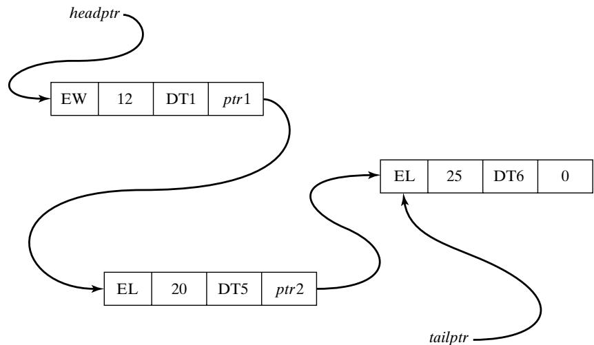 Figure 9 The dump-truck future event list as a linked list.
General Principles
so that
R next eventtype = EL
R next eventtime = 20
R next next is the pointer to the third event notice on the FEL
If one of the pointer fields is zero (or null), then that record is the last item in the list, and the pointer variable tailptr points to that last record, as depicted in Figure 9.
What we have described are called singly-linked lists, because there is a one-way linkage from the head of the list to its tail. The tail pointer is kept mostly for convenience and efficiency, especially for lists for which items are added at the bottom of the list. Of course, a tail pointer is not strictly necessary, because the last item can always be found by traversing the list, but it does make some operations more efficient.
For some purposes, it is desirable to traverse or search a list by starting at the tail in addition to the head. For such purposes, a doubly-linked list can be used. Records on a doubly-linked list have two pointer fields, one for the next record and one for the previous record. Good references that discuss arrays, singly- and doubly-linked lists, and searching and traversing of lists are Cormen, et al. [2001] and Sedgewick [1998].
2.4 Advanced Techniques
Many of the modern simulation packages use techniques and representations of lists that are more efficient than searching through a doubly-linked list. Most of these topics are too advanced for this text. The purpose of this section is to introduce some of the more advanced ideas briefly.
One idea to speed up processing of doubly-linked lists is to use a middle pointer in addition to a head and tail pointer. With special techniques, the mid pointer will always point to the approximate middle of the list. Then, when a new record is being added to the list, the algorithm first examines the middle record to decide whether to begin searching at the head of the list or the middle of the list. Theoretically, except for some overhead due to maintenance of the mid pointer, this technique should cut search times in half. A few advanced techniques use one or more mid pointers, depending on the length of the list
Some advanced algorithms use list representations other than a doubly-linked list, such as heaps or trees. These topics are beyond the scope of this text. Good references are Cormen, et al. [2001] and Sedgewick [1998].
3 Summary
This chapter introduced the major concepts and building blocks in simulation, the most important being entities and attributes, events, and activities. The three major world views—event scheduling, process interaction, activity scanning—were discussed. Finally, to gain an understanding of one of the most important underlying methodologies, Section 2 introduced some of the basic notions of lis processing.
REFERENCES
CORMEN, T. H., C. E. LEISEROON,AND R. L. RIVEST [2001], Introduction toAlgorithms, 2nd ed., McGraw-Hill, New York.
SCHRIBER, T. J., AND D. T. BRUNNER [2003], “Inside Simulation Software: How it Works and Why it Matters,” Proceedings of the 2003 Winter Simulation Conference, S. Chick, P. J. S´anchez, D. Ferrin, and D. J. Morrice, eds., New Orleans, LA, Dec. 7–10, pp. 113–123.
SEDGEWICK, R. [1998], Algorithms in C , 3d ed., Addison-Wesley, Reading, MA.
EXERCISES
Instructions to the reader: For most exercises, the reader should first construct a model by explicitly defining the following:
system state;
system entities and their attributes;
sets, and the entities that may be put into the sets;
events and activities; event notices;
variables needed to collect cumulative statistics.
Second, the reader should either (1) develop the event logic (as in Figures 5 and 6 for Example 3) in preparation for using the event-scheduling approach, or (2) develop the system processes (as in Figure 4) in preparation for using the process-interaction approach.
Most problems contain activities that are uniformly distributed over an interval [a, b]. When conducting a manual simulation, assume that are the only possible values; that is, the activity time is a discrete random variable. The discreteness assumption will simplify the manual simulation.
- (a) Using the event-scheduling approach, continue the (manual) checkout-counter simulation in Example 3, Table 1. Use the same interarrival and service times that were previously generated and used from the Simulation Examples in a Spreadsheet chapter in Table 11, the simulation table for Example 5. (This refers to columns C and E of Table 11.) Continue until all arriving customers receive service.After using the last interarrival time, assume there are no more arrivals.
(b) Do exercise 1(a) again, adding the model components necessary to estimate mean response time and proportion of customers who spend 5 or more minutes in the system. [Hint: See Example 4, Table 2.]
(c) Comment on the relative merits of manual versus computerized simulations.
Construct the event-logic diagrams for the dump-truck problem, Example 5.
In the dump-truck problem of Example 5, it is desired to estimate mean response time and the proportion of response times which are greater than 30 minutes. A response time for a truck begins when that truck arrives at the loader queue and ends when the truck finishes weighing. Add the model components and cumulative statistics needed to estimate these two measures of system performance. Simulate for 8 hours.
Prepare a table in the manner of Table 2, until the CLOCK reaches time 15, using the interarriva and service times given below in the order shown. The stopping event will be at time 30.
| Interarrival times: | 1 | 5 | 6 | 3 | 8 |
|---|---|---|---|---|---|
| Service times: | 3 | 5 | 4 | 1 | 5 |
Continue Table 2 until caller C7 departs.
The data for Table 2 are changed to the following:
| Interarrival times: | 4 | 5 | 2 | 8 | 3 | 7 |
|---|---|---|---|---|---|---|
| Service times: | 5 | 3 | 4 | 6 | 2 | 7 |
Prepare a table in the manner of Table 2 with a stopping event at time 25.
Redo Example 6 from the Simulation Examples in a Spreadsheet chapter (the Able–Baker cal center problem) by a manual simulation, using the event-scheduling approach.
Redo Example 8 from the Simulation Examples in a Spreadsheet chapter (the (M, N) inventory system) by a manual simulation, using the event-scheduling approach.
Redo Example 9 from the Simulation Examples in a Spreadsheet chapter (the bearing-replacement problem) by a manual simulation, using the event-scheduling approach.
Rework Example 5, but using the following data:
| Loading times: | 10 | 5 | 10 | 10 | 5 | 10 | 5 |
|---|---|---|---|---|---|---|---|
| Weigh times: | 12 | 16 | 12 | 12 | 16 | 12 | 12 |
| Travel times: | 40 | 60 | 40 | 80 | 100 | 40 |