4 Simulation Software
In this chapter, we first discuss the history of simulation software and speculate on its future. Simulation software has a history that is just reaching middle age. We base this history on our collective experience, articles written by Professor Richard Nance, panel discussions at the annual Winter Simulation Conference, and a recent article by one of the co-authors.
Next, we discuss features and attributes of simulation software. If you were about to purchase simulation software, what would concern you? Would it be the cost, the ease of learning, the ease o use, or would it be the power to model the kind of system with which you are concerned? Or would it be the animation capabilities? Following the discussion of features, we discuss other issues and concerns related to the selection of simulation software.
Software used to develop simulation models can be divided into three categories. First, there are the general-purpose programming languages, such as C, C , and Java. Second, there are simulation programming languages, examples being GPSS/H and SIMAN V®. Third, there are the simulation environments. This category includes many products that are distinguished one way or another (by, for example, cost, application area, or type of animation), but have common characteristics, such as a graphical user interface and an environment that supports all (or most) aspects of a simulation study. Many simulation environments contain a simulation programming language, but some take a graphical approach similar to process-flow diagramming.
In the first category, we discuss simulation in Java. Java is a general-purpose programming language that was not specifically designed for use in simulation. Java was chosen since it is widely
used and widely available. Today very few people writing discrete-event simulation models are using programming languages alone; however, in certain application areas, some people are using packages based on Java or on some other general-purpose language. Understanding how to develop a model in a general-purpose language helps to understand how basic concepts and algorithms are implemented.
In the second category, we discuss GPSS/H, a highly structured process-interaction simulation language. GPSS was designed for relatively easy simulation of queueing systems, as in job shops, but it has been used to simulate systems of great complexity. It was first introduced by IBM; today, there are various implementations of GPSS, GPSS/H being one of the most widely used.
In the third category, we have selected a number of simulation software packages for discussion. There are many simulation packages currently available; we have selected a few that have survived and thriven for a number of years, to represent different approaches for model building.
One of the important components of a simulation environment is the output analyzer, which is used to conduct experimentation and assist with analyses. To illustrate the range of desirable characteristics, we look at four tools incorporated into some of the simulation environments. Typically these statistical analysis tools compute summary statistics, confidence intervals, and other statistica measures. Some support warmup determination, design of experiments, and sensitivity analyses. Many packages now offer optimization techniques based on genetic algorithms, evolutionary strategies, tabu search, scatter search, and other recently developed heuristic methods. In addition to the support for statistical analysis and optimization, the simulation environments offer data management, scenario definition, and run management. Data management offers support for managing all the inpu and output data associated with the analyses.
1 History of Simulation Software
Our discussion of the history of simulation software is based on Nance [1995], who breaks the years from 1955 through 1986 into five periods. Additional historical information is taken from a panel discussion at the 1992 Winter Simulation Conference entitled “Perspectives of the Founding Fathers” [Wilson et al., 1992], during which eight early users of simulation presented their historica perspectives. We add a sixth and most recent period, and then speculate on the future:
1955–1960 The Period of Search
1961–1965 The Advent
1966–1970 The Formative Period
1971–1978 The Expansion Period
1979–1986 The Period of Consolidation and Regeneration
1987–2008 The Period of Integrated Environments
2009–2011 The Future
The following subsections provide a brief presentation of this history. As indicated in Nance [1995], there were at least 137 simulation programming languages reported as of 1981, and many more since then. This brief history is far from comprehensive. The languages and packages we mention have stood the test of time by surviving to the present day or were the historical forerunner of a package in present use.
1.1 The Period of Search (1955–1960)
In the early years, simulation was conducted in FORTRAN or other general-purpose programming language, without the support of simulation-specific routines. In their first period, much effort was expended on the search for unifying concepts and the development of reusable routines to facilitate simulation. The General Simulation Program of K.D. Tocher and D.G. Owen [1960] is considered the first “language effort.” Tocher identified and developed routines that could be reused in subsequent simulation projects.
1.2 The Advent (1961–1965)
The forerunners of the simulation programming languages (SPLs) in use today appeared in the period 1961–1965. As Harold Hixson said in Wilson et al., [1992], “in the beginning there were FORTRAN, ALGOL, and GPSS”—that is, there were the FORTRAN-based packages (such as SIMSCRIPT and GASP), the ALGOL descendent SIMULA, and GPSS.
The first process-interaction SPL, GPSS was developed by Geoffrey Gordon at IBM and appeared in about 1961. Gordon developed GPSS (General Purpose Simulation System) for quick simulations of communications and computer systems, but its ease of use quickly spread its popularity to other application areas. GPSS is based on a block-diagram representation (similar to a process-flow diagram) and is suited for queueing models of all kinds. As reported by Reitman in Wilson et al., [1992], as early as 1965 GPSS was connected to an interactive display terminal that could interrup and display intermediate results, a foreshadowing of the interactive simulations of today, but far too expensive at the time to gain widespread use.
Harry Markowitz (later to receive a Nobel Prize for his work in portfolio theory) provided the major conceptual guidance for SIMSCRIPT, first appearing in 1963. The RAND Corporation developed the language under sponsorship of the U.S. Air Force. SIMSCRIPT originally was heavily influenced by FORTRAN, but in later versions, its developers broke from its FORTRAN base and created its own SPL. The initial versions were based on event scheduling.
Phillip J. Kiviat of theApplied Research Laboratory of the United States Steel Corporation began the development of GASP (General Activity Simulation Program) in 1961. Originally, it was based on the general-purpose programming language ALGOL, but later a decision was made to base it on FORTRAN. GASP, like GPSS, used flowchart symbols familiar to engineers. It was not a language proper, but rather a collection of FORTRAN routines to facilitate simulation in FORTRAN.
Numerous other SPLs were developed during this time. Notably, they included SIMULA, an extension of ALGOL, developed in Norway and widely used in Europe, and the Control and Simulation Language (CSL), which took an activity-scanning approach.
1.3 The Formative Period (1966–1970)
During this period, concepts were reviewed and refined to promote a more consistent representation of each language’s worldview. The major SPLs matured and gained wider usage.
Rapid hardware advancements and user demands forced some languages, notably GPSS, to undergo major revisions. GPSS/360, with its extensions to earlier versions of GPSS, emerged for the IBM 360 computer. Its popularity motivated at least six other hardware vendors and other groups to produce their own implementations of GPSS or a look-alike.
SIMSCRIPT II represented a major advancement in SPLs. In its free-form English-like language and “forgiving” compiler, an attempt was made to give the user major consideration in the language design.
ECSL, a descendent of CSL, was developed and became popular in the UK. In Europe, SIMULA added the concept of classes and inheritance, thus becoming a precursor of the modern object-oriented programming languages.
1.4 The Expansion Period (1971–1978)
Major advances in GPSS during this period came from outside IBM. Julian Reitman of Norden Systems headed the development of GPSS/NORDEN, a pioneering effort that offered an interactive, visual online environment. James O. Henriksen of Wolverine Software developed GPSS/H, released in 1977 for IBM mainframes, later for mini-computers and the PC. It was notable for being compiled and reportedly 5 to 30 times faster than standard GPSS. With the addition of new features, including an interactive debugger, it has become the principal version of GPSS in use today.
Alan Pritsker at Purdue made major changes to GASP, with GASP IV appearing in 1974. It incorporated state events in addition to time events, thus adding support for the activity-scanning worldview in addition to the event-scheduling worldview.
Efforts were made during this period to try and simplify the modeling process. Using SIMULA, an attempt was made to develop a system definition from a high-level user perspective that could be translated automatically into an executable model. Similar efforts included interactive program generators, the “Programming by Questionnaire,” and natural-language interfaces, together with automatic mappings to the language of choice. As did earlier over-optimistic beliefs in automatic programming, these efforts ran into severe limitations in the generality of what could be modeled— that is, they ran into the unavoidable complexity of real-world systems. Nevertheless, efforts to simplify simulation modeling continue, with the most success seen in simulation systems designed for application to narrow domains.
1.5 The Period of Consolidation and Regeneration (1979–1986)
The fifth period saw the beginnings of SPLs written for, or adapted to, desktop computers and the microcomputer. During this period, the predominant SPLs extended their implementations to many computers and microprocessors while maintaining their basic structure.
Two major descendants ofGASP appeared: SLAM II and SIMAN. The Simulation Language for Alternative Modeling (SLAM), produced by Pritsker and Associates, Inc., sought to provide multiple modeling perspectives and combined modeling capabilities [Pritsker and Pegden, 1979]—that is, it had an event-scheduling perspective based on GASP, a network worldview (a variant of the processinteraction perspective), and a continuous component. With SLAM, you could select one worldview or use a mix of all three.
SIMAN (SIMulation ANalysis) possessed a general modeling capability found in SPLs such as GASP IV, but also had a block-diagram component similar in some respects to that in SLAM and GPSS. C. Dennis Pegden developed SIMAN as a one-person faculty project over a period o about two years; he later founded Systems Modeling Corporation to market SIMAN. SIMAN was the first major simulation language executable on the IBM PC and designed to run under MS-DOS constraints. Similar to GASP, SIMAN allowed an event-scheduling approach by programming in FORTRAN with a supplied collection of FORTRAN routines, a block-diagram approach (another variant of the process-interaction worldview) analogous in some ways to that of GPSS and SLAM, and a continuous component.
1.6 The Period of Integrated Environments (1987–2008)
This period is notable for the growth of SPLs on the personal computer and the emergence of simulation environments with graphical user interfaces, animation, and other visualization tools. AutoMod and Extend were two of the earliest software packages to offer integrated simulation environments. Today, virtually all simulation packages come with environments that integrate model building, model debugging, animation, and interactive running of models. Many of these environments also contain input-data analyzers and output analyzers. Some packages attempt to simplify the modeling process by the use of process-flow or block diagramming and of “fill-in-the-blank” windows that avoid the need to learn programming syntax. Animation ranges from schematic-like representations to 2-D and 3-D scale drawings.
Recent advancements have been made in web-based simulation. Simulation has been deemed to have a role in supply-chain management. The combination of simulation and emulation shows promise. (Emulation is the imitation of a device such as those material handling devices illustrated in www.demo3d.com.)
1.7 The Future (2009–2011)
In an article in the ICS Newsletter [Banks, 2008], one ofthe co-authors asked a panel ofsimulationists, including well-known experts in their field, their opinion or best guess regarding future developments in discrete-event simulation. The first question was: “What remarkable results will we observe in simulation software in the near term, say, within three years?”
The most-often mentioned future developments, including more use of virtual reality, included an improved user interface, better animation, and a paradigm shift such as a major adoption o agent-based modeling in discrete-event modeling. Although, to date, agent-based modeling has been widely used in modeling collective behavior (civil violence, war, even determining what elements cause a standing ovation) and social phenomenon (seasonal migration, pollution, transmission of disease, and sexual reproduction, to name a few) its use in industrial and commercial simulations is just beginning.
Agent-based modeling is a method for simulating the actions and interactions of autonomous individuals (the agents) in a network, with a view to assessing their effects on the system as a whole. Agents may be people or animals or other entities that have agency, meaning that they are not passive, they actively make decisions, retain memory of past situations and decisions, and exhibit learning. In summary, agents are active and may exhibit cognition, memory, and learning. They may or may not be goal-directed.
Each agent’s behavior is governed by a set oflocal rules; that is, the agent responds in a prescribed way to local, near-by conditions. The interest is in patterns of behavior that emerge for the group of agents, called emergent behavior.
An interesting and well known example is the “boids” (that is, simulated birds flying in a given 2-D or 3-D area) in which flocking behavior emerges. (You can find many examples of the boids model on the Internet, each based on similar but not identical assumptions or rules. For one, see www.navgen.com/3d boids.) The flocking behavior is not scripted or explicitly programmed, but rather it emerges naturally (and somewhat surprisingly) from a set of fairly simple rules. The basic rule is that if a boid comes close to one or more other boids, then it adjusts its direction and speed to the other boids. In most of the boids simulations found on the Internet, the boids are no goal-directed; that is, they have no destination but simply fly. In at least one boids example, the boids do have a goal; there are two or more flocks of boids, and members of one flock attack and kil members of other flocks.
Software packages and toolkits for agent-based modeling include
AnyLogic (www.xjtek.com) discussed in Section 7.1,
Ascape (www.nutechsolutions.com),
MASON (cs.gmu.edu/%7Eeclab/projects/mason),
• NetLogo (ccl.northwestern.edu/netlogo),
StarLogo (education.mit.edu/starlogo),
Swarm (www.swarm.org), and
RePast (www.repast.sourceforge.net),
to name a few.
Information about various software packages is given in Section 7, including the websites of the vendors. A view of current developments in simulation software is available from these websites.
2 Selection of Simulation Software
This chapter includes a brief introduction to a number of simulation-software packages. Every two years, the journal OR/MS Today publishes a simulation-software survey [Swain, 2007]. The 2007 issue had 48 products, including simulation support packages such as input-data analyzers.
There are many features that are relevant when selecting simulation software [Banks, 1996]. Some of these features are shown, along with a brief description, in Tables 1 to 5. We offer the following advice when evaluating and selecting simulation software:
Do not focus on a single issue, such as ease of use. Consider the accuracy and level of detai obtainable, ease of learning, vendor support, and applicability to your applications.
Execution speed is important. Do not think exclusively in terms of experimental runs that take place at night and over the weekend. Speed affects development time. During debugging, an analyst might have to wait for the model to run up to the point in simulated time where an error occurs many times before the error is identified.
Beware of advertising claims and demonstrations. Many advertisements exploit positive features of the software only. Similarly, the demonstrations solve the test problem very well, but perhaps not your problem.
Ask the vendor to solve a small version of your problem.
Ta ble 1 M od e l - B _u i l d i n _g Feat_u res
| Feature | Description |
|---|---|
| Modeling worldview | Process interaction, event perspectives, and continuous modeling, depending on needs |
| Input-data analysis capability | Estimate empirical or statistical distributions from raw data |
| Graphical model building | Process-flow, block-diagram, or network approach |
| Conditional routing | Route entities based on prescribed conditions or attributes |
| Simulation programming | Capability to add procedural logic through a high-level powerful simulation language |
| Syntax | Easily understood, consistent, unambiguous, English-like |
| Input flexibility | Accepts data from external files, databases, spreadsheets, or interactively |
| Modeling conciseness | Powerful actions, blocks, or nodes |
| Randomness | Random-variate generators for all common distributions, e.g., exponential triangular uniform normal |
| Specialized components and templates | Material handling: vehicles, conveyors, bridge cranes, AS/RS, etc. Handling of liquids and bulk materials Communication systems Computer systems Call centers Others |
| User-built custom objects | Reusable objects, templates, and submodels |
| Continuous flow | Tanks and pipes or bulk conveyors |
| Interface with general-programming language | Link code in C, C++, Java, or other general-programming language |
Table 2 Runtime Environment
| Feature | Description |
|---|---|
| Execution speed | Many runs needed for scenarios and replications. Impacts development as well as experimentation |
| Model size; number of variables and attributes | Should have no built-in limits |
| Interactive debugger | Monitor the simulation in detail as it progresses. Ability to break, trap, run until, step; to display status, attributes and variables; etc. |
| Model status and statistics | Display at any time during simulation |
| Runtime license | Ability to change parameters and run a model (but not to change logic or build a new model) |
- Beware of “checklists” with “yes” and “no” as the entries. For example, many packages claim to have a conveyor entity. However, implementations have considerable variation and leve of fidelity. Implementation and capability are what is important. As a second example, mos packages offer a runtime license, but these vary considerably in price and features.
Table 3 Animation and Layout Features
| Feature | Description |
|---|---|
| Type of animationImport drawing and object files | True to scale or iconic (such as process-flow diagram)From CAD (vector formats) drawings or icons (bit-mapped or raster graphics) |
| Dimension | 2-D, 2-D with perspective, 3-D |
| Movement | Motion of entities or status indicators |
| Quality of motion | Smooth or jerky |
| Libraries of common objects | Extensive predrawn graphics |
| Navigation | Panning, zooming, rotation |
| Views | User defined, named |
| Display step | Control of animation speed |
| Selectable objects | Dynamic status and statistics displayed upon selection |
| Hardware requirements | Standard or special video card |
Table 4 Output Features
| Feature | Description |
|---|---|
| Scenario manager | Create user-defined scenarios to simulate |
| Run manager | Make all runs (scenarios and replications) and save results for future analyses |
| Warmup capability | For steady-state analysis |
| Independent replications | Using a different set of random numbers |
| Optimization | Genetic algorithms, tabu search, etc. |
| Standardized reports | Summary reports including averages, counts, minimum and maximum, etc. |
| Customized reports | Tailored presentations for managers |
| Statistical analysis | Confidence intervals, designed experiments, etc. |
| Business graphics | Bar charts, pie charts, time lines, etc. |
| Costing module | Activity-based costing included |
| File export | Input to spreadsheet or database for custom processing and analysis |
| Database maintenance | Store output in an organized manner |
Table 5 Vendor Support and Product Documentation
| Feature | Description |
|---|---|
| Training | Regularly scheduled classes of high quality |
| Documentation | Quality, completeness, online |
| Help system | General or context-sensitive |
| Tutorials | For learning the package or specific features |
| Support | Telephone, e-mail, web |
| Upgrades, maintenance | Regularity of new versions and maintenance releases that address customer needs |
| Track record | Stability, history, customer relations |
Simulation users ask whether the simulation model can link to and use code or routines written in external languages such as C, C , or Java. This is a good feature, especially when the external routines already exist and are suitable for the purpose at hand. However, the more important question is whether the simulation package and language are sufficiently powerful to avoid having to write logic in any external language.
There may be a significant trade-off between the graphical model-building environments and ones based on a simulation language. Graphical model building removes the learning curve
due to language syntax, but it does not remove the need for procedural logic in most realworld models and the debugging to get it right. Beware of “no programming required” unless either the package is a near-perfect fit to your problem domain or programming (customized procedural logic) is possible with the supplied blocks, nodes, or process-flow diagram—in which case “no programming required” refers to syntax only and not the development of procedural logic.
3 An Example Simulation
Example 1: The Checkout Counter: A Typical Single-Server Queue
The system, a grocery checkout counter, is modeled as a single-server queue. The simulation will run until 1000 customers have been served. In addition, assume that the interarrival times of customers are exponentially distributed with a mean of 4.5 minutes, and that the service times are (approximately) normally distributed with a mean of 3.2 minutes and a standard deviation of 0.6 minute. (The approximation is that service times are always positive.) When the cashier is busy, a queue forms with no customers turned away. This example was simulated manually by using the event-scheduling point of view. The model contains two events: the arrival and departure events.
The following three sections illustrate the simulation ofthis single-server queue in Java, GPSS/H, and SSF (Scalable Simulation Framework). Although this example is much simpler than models that arise in the study of complex systems, its simulation contains the essential components of all discrete-event simulations.
4 Simulation in Java
Java is a widely available programming language that has been used extensively in simulation. It does not, however, provide any facilities directly aimed at aiding the simulation analyst, who therefore must program all details of the event-scheduling/time-advance algorithm, the statistics-gathering capability, the generation ofsamples from specified probability distributions, and the report generator. Nevertheless, the runtime library does provide a random-number generator. Unlike FORTRAN or C, the object-orientedness of Java does support modular construction of large models. For the mos part, the special-purpose simulation languages hide the details of event scheduling, whereas in Java all the details must be explicitly programmed. To a certain extent though, simulation libraries such as SSF [Cowie, 1999] alleviate the development burden by providing access to standardized simulation functionality and by hiding low-level scheduling minutiae.
There are many online resources for learning Java; we assume a prior working knowledge of the language. Any discrete-event simulation model written in Java contains the components discussed in Section 3: system state, entities and attributes, sets, events, activities and delays, and the components listed below. To facilitate development and debugging, it is best to organize the Java model in a modular fashion by using methods. The following components are common to almost all models written in Java:
Clock A variable defining simulated time
Initialization method A method to define the system state at time 0
Min-time event method A method that identifies the imminent event, that is, the element of the future event list (FutureEventList) that has the smallest time-stamp
Event methods For each event type, a method to update system state (and cumulative statistics) when that event occurs
Random-variate generators Methods to generate samples from desired probability distributions
Main program To maintain overall control of the event-scheduling algorithm
Report generator A method that computes summary statistics from cumulative statistics and prints a report at the end of the simulation
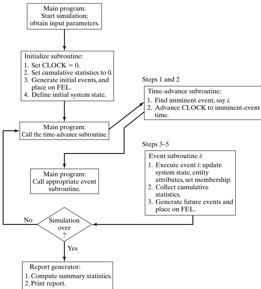 Figure 1 Overall structure of an event-scheduling simulation program.
The overall structure of a Java simulation program is shown in Figure 1.
The simulation begins by setting the simulation Clock to zero, initializing cumulative statistics to zero, generating any initial events (there will always be at least one) and placing them on the FutureEventList, and defining the system state at time 0. The simulation program then cycles, repeatedly passing the current least-time event to the appropriate event methods until the simulation is over.At each step, after finding the imminent event but before calling the event method, the simulation Clock is advanced to the time of the imminent event. (Recall that, during the simulated time between the occurrence of two successive events, the system state and entity attributes do not change in value. Indeed, this is the definition of discrete-event simulation: The system state changes only when an event occurs.) Next, the appropriate event method is called to execute the imminent event, update cumulative statistics, and generate future events (to be placed on the FutureEventList). Executing the imminent event means that the system state, entity attributes, and set membership are changed to reflect the fact that the event has occurred. Notice that all actions in an event method take place a one instant of simulated time. The value of the variable Clock does not change in an event method. If the simulation is not over, control passes again to the time-advance method, then to the appropriate event method, and so on. When the simulation is over, control passes to the report generator, which computes the desired summary statistics from the collected cumulative statistics and prints a report.
The efficiency of a simulation model in terms of computer runtime is determined to a large extent by the techniques used to manipulate the FutureEventList and other sets. As discussed earlier in Section 3, removal of the imminent event and addition of a new event are the two main operations performed on the FutureEventList. Java includes general, efficient data structures for searching and priority lists; it is usual to build a customized interface to these to suit the application. In the example to follow, we use customized interfaces to implement the event list and the list o waiting customers. The underlying priority-queue organization is efficient, in the sense of having access costs that grow only in the logarithm of the number of elements in the list.
Example 2: Single-Server Queue Simulation in Java
The grocery checkout counter, defined in detail in Example 1, is simulated by using Java.
Class Event represents an event. It stores a code for the event type (arrival or departure), and the event time-stamp. It has associated methods (functions) for creating an event and accessing its data. It also has an associated method compareTo, which compares the event with another (passed as an argument) and reports whether the first event should be considered to be smaller, equal, or larger than the argument event. The methods for this model and the flow of control are shown in Figure 2, which is an adaptation of Figure 1 for this particular problem. Table 6 lists the variables used for system state, entity attributes and sets, activity durations, and cumulative and summary statistics; the functions used to generate samples from the exponential and normal distributions; and all the other methods needed.
Table 6 Definitions of Variables, Functions, and Methods in the Java Model of the Single-Server Queue
| Variables | Description |
|---|---|
| System state | |
| QueueLength | Number of customers queued (but not in service) at current simulated time |
| NumberInService | Number being served at current simulated time |
| Entity attributes and sets | |
| Customers | FCFS queue of customers in system |
| Future event list | |
| FutureEventList | Priority-ordered list of pending events |
| Activity durations | |
| MeanInterArrivalTime | The interarrival time between the previous customer’s arrival and the next arrival |
| MeanServiceTime | The service time of the most recent customer to begin service |
| Input parameters | |
| MeanInterarrivalTime | Mean interarrival time (4.5 minutes) |
| MeanServiceTime | Mean service time (3.2 minutes) |
| SIGMA | Standard deviation of service time (0.6 minute) |
| TotalCustomers | The stopping criterion—number of customers to be served (1000) |
| Simulation variables | |
| Clock | The current value of simulated time |
| Statistical Accumulators | |
| LastEventTime | Time of occurrence of the last event |
| TotalBusy | Total busy time of server (so far) |
| MaxQueueLength | Maximum length of waiting line (so far) |
| SumResponseTime | Sum of customer response times for all customers who have departed (so far) |
| NumberOfDepartures | Number of departures (so far) |
| LongService | Number of customers who spent 4 or more minutes at the checkout counter (so far) |
| Summary statistics | |
| RHO =BusyTime/Clock | Proportion of time server is busy (here the value of Clock is the final value of simulated time) |
| AVGR | Average response time (equal to SumResponseTime/TotalCustomers) |
| PC4 | Proportion of customers who spent 4 or more minutes at the checkout counter |
| Functions | Description |
| exponential(mu)normal(xmu, SIGMA) | Function to generate samples from an exponential distribution with mean muFunction to generate samples from a normal distribution with mean xmu and standard deviation SIGMA |
| Methods | Description |
| InitializationProcessArrivalProcessDepartureReportGeneration | Initialization methodEvent method that executes the arrival eventEvent method that executes the departure eventReport generator |
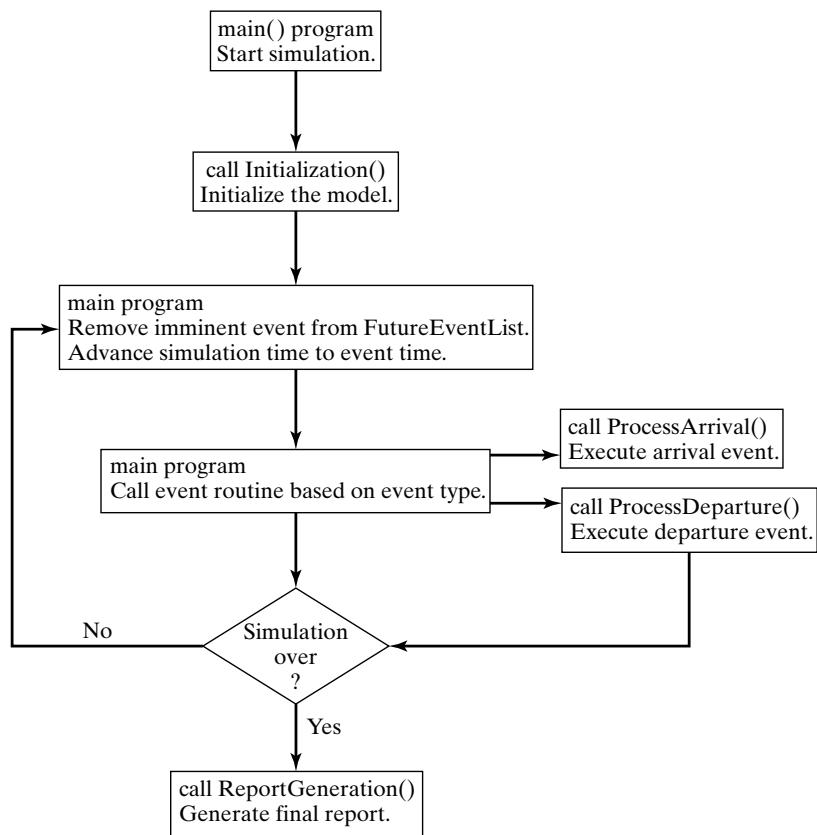 Figure 2 Overall structure of Java simulation of a single-server queue.
Figure 3 Java main program for the single-server queue simulation.
The entry point of the program and the location of the control logic is through class Sim, shown in Figure 3. Variables of classes EventList and Queue are declared. As these classes are all useful for programs other than Sim, their declarations are given in other files, per Java rules. A variable of the Java built-in class Random is also declared; instances of this class provided randomnumber streams. The main method controls the overall flow of the event-scheduling/time-advance algorithm.
Figure 4 Java initialization method for the single-server queue simulation.
The main program method first gives values to variables describing model parameters; it creates instances of the random-number generator, event list, and customer queue; and then it calls method Initialization to initialize other variables, such as the statistics-gathering variables. Contro then enters a loop which is exited only after TotalCustomers customers have received service. Inside the loop, a copy of the imminent event is obtained by calling the getMin method of the priority queue, and then that event is removed from the event list by a call to dequeue. The globa simulation time Clock is set to the time-stamp contained in the imminent event, and then either ProcessArrival or ProcessDeparture is called, depending on the type of event. When the simulation is finally over, a call is made to method ReportGeneration to create and print out the final report.
A listing for the Sim class method Initialization is given in Figure 4. The simulation clock, system state, and other variables are initialized. Note that the first arrival event is created by generating a local Event variable whose constructor accepts the event’s type and time. The even time-stamp is generated randomly by a call to Sim class method exponential and is passed to the random-number stream to use with the mean of the exponential distribution from which to sample. The event is inserted into the future event list by calling method enqueue. This logic assumes tha the system is empty at simulated time Clock 0, so that no departure can be scheduled. It is straightforward to modify the code to accommodate alternative starting conditions by adding events to FutureEventList and Customers as needed.
Figure 5 gives a listing of Sim class method ProcessArrival, which is called to process each arrival event. The basic logic of the arrival event for a single-server queue (where LQ corresponds to QueueLength and LS corresponds to NumberInService). First, the new arrival is added to the queue Customers of customers in the system. Next, if the server is idle (NumberInService 0) then the new customer is to go immediately into service, so Sim class method ScheduleDeparture is called to do that scheduling. An arrival to an idle queue does no update the cumulative statistics, except possibly the maximum queue length. An arrival to a busy queue does not cause the scheduling of a departure, but does increase the total busy time by the amount of simulation time between the current event and the one immediately preceding it (because, if the server is busy now, it had to have had at least one customer in service by the end of processing the previous event). In either case, a new arrival is responsible for scheduling the nex arrival, one random interarrival time into the future. An arrival event is created with simulation time equal to the current Clock value plus an exponential increment, that event is inserted into the future event list, the variable LastEventTime recording the time of the last event processed is set to the current time, and control is returned to the main method of class Sim.
Figure 5 Java arrival event method for the single-server queue simulation.
Sim class method ProcessDeparture, which executes the departure event, is listed in Figure 6, as is method ScheduleDeparture. After removing the event from the queue of al customers, the number in service is examined. If there are customers waiting, then the departure of the next one to enter service is scheduled. Then, cumulative statistics recording the sum of al response times, sum of busy time, number of customers who used more than 4 minutes of service time, and number of departures are updated. (Note that the maximum queue length cannot change in value when a departure occurs.) Notice that customers are removed from Customers in FIFO order; hence, the response time response of the departing customer can be computed by subtracting the arrival time of the job leaving service (obtained from the copy of the arrival event removed from the Customers queue) from the current simulation time. After the incrementing of the total number o departures and the saving of the time of this event, control is returned to the main program.
Figure 6 also gives the logic of method ScheduleDeparture, called by both Process-Arrival and ProcessDeparture to put the next customer into service. The Sim class method normal, which generates normally distributed service times, is called until it produces a nonnegative sample. A new event with type departure is created, with event time equal to the current simulation time plus the service time just sampled. That event is pushed onto FutureEventList, the number
Figure 6 Java departure event method for the single-server queue simulation.
in service is set to one, and the number waiting (QueueLength) is decremented to reflect the fact that the customer entering service is waiting no longer.
The report generator, Sim class method ReportGeneration, is listed in Figure 7. The summary statistics, RHO, AVGR, and PC4, are computed by the formulas in Table 6; then the input parameters are printed, followed by the summary statistics. It is a good idea to print the input parameters at the end of the simulation, in order to verify that their values are correct and that these values have not been inadvertently changed.
Figure 8 provides a listing of Sim class methods exponential and normal, used to generate random variates. Both of these functions call method nextDouble, which is defined for the built-in Java Random class generates a random number uniformly distributed on the (0,1) interval. We use Random here for simplicity of explanation; superior random-number generators can be built by hand. The techniques for generating exponentially and normally distributed random variates are based on first generating a U(0,1) random number.
The output from the grocery-checkout-counter simulation is shown in Figure 9. It should be emphasized that the output statistics are estimates that contain random error. The values shown are influenced by the particular random numbers that happened to have been used, by the initia conditions at time 0, and by the run length (in this case, 1000 departures).
Figure 7 Java report generator for the single-server queue simulation.
In some simulations, it is desired to stop the simulation after a fixed length of time, say TE 12 hours 720 minutes. In this case, an additional event type, stop event, is defined and is scheduled to occur by scheduling a stop event as part of simulation initialization. When the stopping event does occur, the cumulative statistics will be updated and the report generator called. The main program and method Initialization will require minor changes. Exercise 1 asks the reader to make these changes. Exercise 2 considers the additional change that any customer at the checkout counter at simulated time Clock TE should be allowed to exit the store, but no new arrivals are allowed after time TE.
Figure 8 Random-variate generators for the single-server queue simulation.
Figure 9 Output from the Java single-server queue simulation.
5 Simulation in GPSS
GPSS is a highly structured, special-purpose simulation programming language based on the processinteraction approach and oriented toward queueing systems. A block diagram provides a convenien way to describe the system being simulated. There are over 40 standard blocks in GPSS. Entities called transactions may be viewed as flowing through the block diagram. Blocks represent events, delays, and other actions that affect transaction flow. Thus, GPSS can be used to model any situation where transactions (entities, customers, units of traffic) are flowing through a system (e.g., a network of queues, with the queues preceding scarce resources). The block diagram is converted to block statements, control statements are added, and the result is a GPSS model.
The first version of GPSS was released by IBM in 1961. It was the first process-interaction simulation language and became popular; it has been implemented anew and improved by many parties since 1961, with GPSS/H being the most widely used version today. Example 3 is based on GPSS/H.
GPSS/H is a product ofWolverine Software Corporation, www.wolverinesoftware.com [Banks, Carson, and Sy, 1995; Henriksen, 1999]. It is a flexible, yet powerful tool for simulation. Unlike the original IBM implementation, GPSS/H includes built-in file and screen I/O, use of an arithmetic expression as a block operand, an interactive debugger, faster execution, expanded contro statements, ordinary variables and arrays, a floating-point clock, built-in math functions, and built-in random-variate generators.
The animator for GPSS/H is ProofAnimation™, another product of Wolverine Software Corporation [Henriksen, 1999]. ProofAnimation provides a 2-D or 3-D animation, usually based on a scale drawing. It can run in postprocessed mode (after the simulation has finished running) or concurrently. In postprocessed mode, the animation is driven by two files: the layout file for the static background, and a trace file that contains commands to make objects move and produce other dynamic events. It can work with any simulation package that can write the ASCII trace file. Alternately, it can run concurrently with the simulation by sending the trace file commands as messages, or it can be controlled directly by using its DLL (dynamic link library) version.
Example 3: Single-Server Queue Simulation in GPSS/H
Figure 10 exhibits the block diagram and Figure 11 the GPSS program for the grocery-store checkoutcounter model described in Example 2. Note that the program (Figure 11) is a translation of the block diagram together with additional definition and control statements. (In the discussion that follows, all nonreserved words are shown in italics.)
In Figure 10, the GENERATE block represents the arrival event, with the interarrival times specified by RVEXPO(1,&IAT). RVEXPO stands for “random variable, exponentially distributed,” the 1 indicates the random-number stream to use, and &IAT indicates that the mean time for the exponential distribution comes from a so-called ampervariable &IAT. Ampervariable names begin with the “&” character; Wolverine added ampervariables to GPSS because the original IBM implementation had limited support for ordinary global variables, with no user freedom for naming them.
The next block is a QUEUE with a queue named SYSTIME. It should be noted that the QUEUE block is not needed for queues or waiting lines to form in GPSS. The true purpose of the QUEUE block is to work in conjunction with the DEPART block to collect data on queues or any other subsystem. In Example 3, we want to measure the system response time—that is, the time a transaction spends in the system. Placing a QUEUE block at the point that transactions enter the system and placing its counterpart the DEPART block, at the point that the transactions complete their processing causes the response times to be collected automatically. The purpose of the DEPART block is to signal the end of data collection for an individual transaction. The QUEUE and DEPART block combination is not necessary for queues to be modeled, but rather is used for statistical data collection.
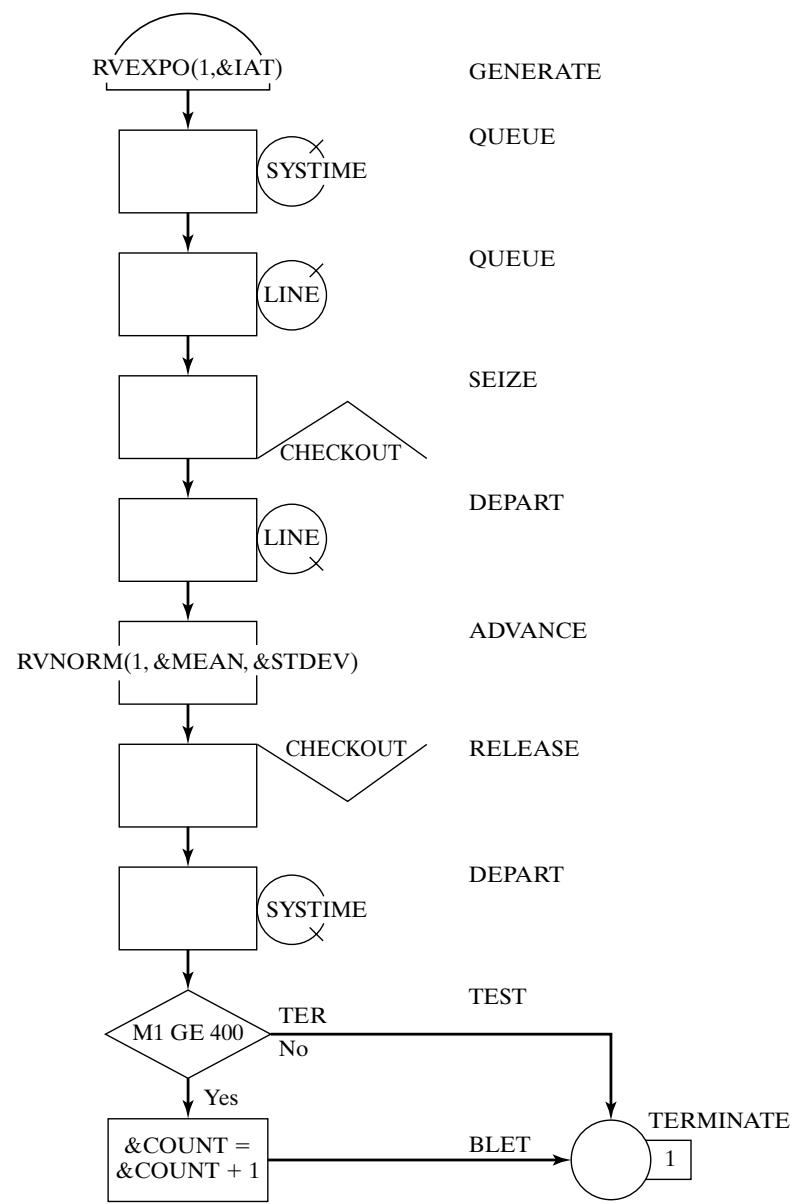 Figure 10 GPSS block diagram for the single-server queue simulation.
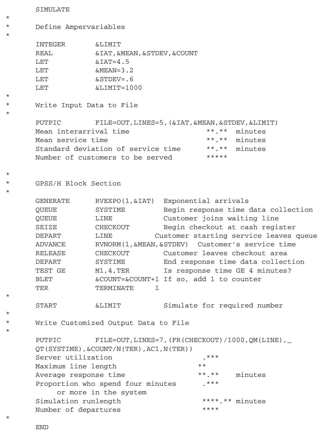 Figure 11 GPSS/H program for the single-server queue simulation.
The next QUEUE block (with queue named LINE) begins data collection for the waiting line before the cashier. The customers may or may not have to wait for the cashier. Upon arrival at an idle checkout counter, or after advancing to the head of the waiting line, a customer captures the cashier, as represented by the SEIZE block with the resource named CHECKOUT. Once the transaction representing a customer captures the cashier represented by the resource CHECKOUT, the data collection for the waiting-line statistics ends, as represented by the DEPART block for the queue named LINE. The transaction’s service time at the cashier is represented by an ADVANCE block. RVNORM indicates “random variable, normally distributed.” Again, random-number stream 1 is being used, the mean time for the normal distribution is given by ampervariable &MEAN, and its standard deviation is given by ampervariable &STDEV. Next, the customer gives up the use o the facility CHECKOUT with a RELEASE block. The end of the data collection for response times is indicated by the DEPART block for the queue SYSTIME.
Next, there is a TEST block that checks to see whether the time in the system, M1, is greater than or equal to 4 minutes. (Note that M1 is a reserved word in GPSS/H; it automatically tracks transaction total time in system.) In GPSS/H, the maxim is “if true, pass through.” Thus, if the customer has been in the system four minutes or longer, the next BLET block (for block LET) adds one to the counter &COUNT. If not true, the escape route is to the block labeled TER. That label appears before the TERMINATE block, whose purpose is the removal of the transaction from the system. The TERMINATE block has a value “1”, indicating that one more transaction is added toward the limiting value (or “transactions to go”).
The control statements in this example are all of those lines in Figure 11 that precede or follow the block section. (There are eleven blocks in the model from the GENERATE block to the TERMINATE block.) The control statements that begin with an “*” are comments, some of which are used for spacing purposes. The control statement SIMULATE tells GPSS/H to conduct a simulation; if it is omitted, GPSS/H compiles the model and checks for errors only. The ampervariables are defined as integer or real by control statements INTEGER and REAL. It seems that the ampervariable &COUNT should be defined as an integer; however, it will be divided later by a real value. If it is integer, the result of an integer divided by a real value is truncation, and that is not desired in this case. The four assignment statements (LET) provide data for the simulation. These four values could have been placed directly into the program; however, the preferred practice is to place them in ampervariables at the top of the program so that changes can be made more easily or the model can be modified to read them from a data file
To ensure that the model data is correct, and for the purpose of managing different scenarios simulated, it is good practice to echo the input data. This is accomplished with a PUTPIC (for “pu picture”) control statement. The five lines following PUTPIC provide formatting information, with the asterisks being markers (called picture formatting) in which the values of the four ampervariables replace the asterisks when PUTPIC is executed. Thus, “**.**” indicates a value that may have two digits following the decimal point and up to two before it.
| Mean interarrival time | 4.50 minutes |
|---|---|
| Mean service time | 3.20 minutes |
| Standard deviation of service time | 0.60 minutes |
| Number of customers to be served | 1000 |
| Server utilization | 0.676 |
| Maximum line length | 7 |
| Average response time | 6.33 minutes |
| Proportion who spend four minutes or more in the system | 0.646 |
| Simulation runlength | 4767.27 minutes |
| Number of departures | 1000 |
Figure 12 Customized GPSS/H output report for the single-server queue simulation.
The START control statement controls simulation execution. It starts the simulation, sets up a “termination-to-go” counter with initial value its operand (&LIMIT), and controls the length of the simulation.
After the simulation completes, a second PUTPIC control statement is used to write the desired output data to the same file OUT. The printed statistics are all gathered automatically by GPSS. The first output in the parenthesized list is the server utilization. FR(CHECKOUT)/1000 indicates tha the fractional utilization of the resource CHECKOUT is printed. Because FR(CHECKOUT) is in parts per thousand, the denominator is provided to compute fractional utilization. QM(LINE) is the maximum value in the queue LINE during the simulation. QT(SYSTIME) is the average time in the queue SYSTIME. &COUNT/N(TER) is the number of customers who had a response time of four or more minutes divided by the number of customers that went through the block with label TER, or N(TER). AC1 is the clock time, whose last value gives the length of the simulation.
The contents of the customized output file OUT are shown in Figure 12. The standard GPSS/H output file is displayed in Figure 13. Although much of the same data shown in the file OUT can be found in the standard GPSS/H output, the customized file is more compact and uses the language of the problem rather than GPSS jargon. There are many other reasons that customized output files are useful. For example, if 50 replications of the model are to be made and the lowest, highest, and average value of a response are desired, this can be accomplished by using control statements, with the results in a very compact form, rather than extracting the desired values from 50 standard outpu files.
6 Simulation in SSF
The Scalable Simulation Framework (SSF) is an Application Program Interface (API) that describes a set of capabilities for object-oriented, process-view simulation. The API is sparse and was designed to allow implementations to achieve high performance (e.g., on parallel computers). SSF APIs exis for both C and Java, and implementations exist in both languages. SSF has a wide user base— particularly in network simulation by using the add-on framework SSFNet (www.ssfnet.org). Our chapter on network simulation uses SSFNet.
| BLOCK CURRENT | TOTAL | BLOCK | CURRENT | TOTAL | ||||||
|---|---|---|---|---|---|---|---|---|---|---|
| 1 | 1003 | TER | 1000 | |||||||
| 2 | 1003 | |||||||||
| 3 | 3 | 1003 | ||||||||
| 4 | 1000 | |||||||||
| 5 | 1000 | |||||||||
| 6 | 1000 | |||||||||
| 7 | 1000 | |||||||||
| 8 | 1000 | |||||||||
| 9 | 1000 | |||||||||
| 10 | 646 | |||||||||
| –AVG-UTIL-DURING– | ||||||||||
| FACILITY | TOTAL | AVAIL | UNAVL | ENTRIES | AVERAGE | CURRENT | PERCENT | SEIZING | PREEMPTING | |
| TIME | TIME | TIME | TIME/XACT | STATUS | AVAIL | XACT | XACT | |||
| CHECKOUT | 0.676 | 1000 | 3.224 | AVAIL | ||||||
| QUEUE | MAXIMUM | AVERAGE | TOTAL | ZERO | PERCENT | AVERAGE | $ AVERAGE | QTABLE | CURRENT | |
| CONTENTS | CONTENTS | ENTRIES | ENTRIES | ZEROS | TIME/UNIT | TIME/UNIT | NUMBER | CONTENTS | ||
| SYSTIME | 8 | 1.331 | 1003 | 0 | 6.325 | 6.235 | 3 | |||
| LINE | 7 | 0.655 | 1003 | 334 | 33.3 | 3.111 | 4.665 | 3 | ||
| RANDOM | ANTITHETIC | INITIAL | CURRENT | SAMPLE | CHI-SQUARE | |||||
| STREAM | VARIATES | POSITION | POSITION | COUNT | UNIFORMITY | |||||
| 1 | OFF | 100000 | 103004 | 3004 | 0.83 |
Fi_g u re 13 Sta n d a rd G PSS/H o ut_p ut re _po rt fo r th e s i n _g l e-se rve r _q u e u e s i m u l at i o n
The SSFAPI defines five base classes. process is a class that implements threads of control; the action method ofa derived class contains the execution body ofthe thread. The Entity class is used to describe simulation objects. It contains state variables, processes, and communication endpoints. The inChannel and outChannel classes are communication endpoints. The Event class defines messages sent between entities. One model entity communicates with another by “writing” an Event into an outChannel; at some later time, it is available at one or more inChannels. A process that expects input on an inChannel can suspend, waiting for an event on it. These points, and others, will be elaborated upon as we work through an SSF implementation of the single-server queue.
Source code given in Figure 14 expresses the logic of arrival generation in SSF for the singleserver queue example. The example is built on two SSF processes. One of these generates jobs and adds them to the system, the other services the enqueued jobs. Class SSQueue is a class tha contains the whole simulation experiment. It uses the auxiliary classes Random (for random-number generation) and Queue (to implement FIFO queueing of general objects). SSQueue defines experimental constants (“public static final” types) and contains SSF communication endpoints out and in, through which the two processes communicate. SSQueue also defines an inner class arrival, which stores the identity and arrival time of each job.
Class Arrivals is an SSF process. Its constructor stores the identity of the entity that owns it, and creates a random-number generator that is initialized with the seed passed to it. For all bu the initial call, method action generates and enqueues a new arrival, then blocks (via SSF method waitFor) for an inter-arrival time; on the first call, it by-passes the job-generation step and blocks for an initial interarrival time. The call to waitFor highlights details needing explanation. An SSQueue object calls the Arrival constructor and is saved as the “owner.” This class contains an auxiliary method exponential, which samples an exponential random variable with specified mean by using a specified random-number stream. It also contains methods d2t and t2d that translate between a discrete “tick”-based integer clock and a double-precision floating-point representation. In the waitFor call, we use the same code seen earlier to sample the exponential in double-precision format, but then use d2t to convert it into the simulator’s integer clock format. The specific conversion factor is listed as an SSQueue constant, 10^9 ticks per unit time.
SSF interprocess communication is used sparingly in this example. Because service is nonpreemptive, when ajob’s service completes, the process providing service can examine the list of waiting customers (in variable owner.Waiting) to see whether it needs to give service to another customer. Thus, the only time the server process needs to be told that there is a job waiting is when a job arrives to an empty system. This is reflected in Arrivals.action by use of its owner’s out channel.
A last point of interest is that Arrivals is, in SSF terminology, a “simple” process. This means that every statement in action that might suspend the process would be the last statement executed under normal execution semantics. The Arrivals class tells SSF that it is simple by overriding a default method isSimple to return the value true, rather than the default value (false). The key reason for using simple processes is performance—they require that no state be saved, only the condition under which the process ought to be reanimated. And, when it is reanimated, it starts executing at the first line of action.
Figure 14 SSF Model of Job-Arrival Process.
Figure 15 illustrates the code for the Server process. Like process Arrival, its constructor is called by an instance of SSQueue and is given the identity of that instance and a random-number seed. Like Arrival, it is a simple process. It maintains state variable in service to remember the specifics of a job in service and state variable service time to remember the value of the service time sampled for the job in service. When the SSF kernel calls action, either a job has completed service, or the Arrival process has just signaled Server though the inChannel. We distinguish the cases by looking at variable in service, which will be nonnull if a job is in service, just now completed. In this case, some statistics are updated. After this task is done, a test is made for customers waiting for service. The first waiting customer is dequeued from the waiting list and is
Figure 15 SSF Model of Single-Server Queue : Server.
copied into the in service variable; the process then samples a service time and suspends through a waitFor call. If no customer was waiting, the process suspends on a waitOn statement until an event from the Arrival process awakens it.
SSF bridges the gap between models developed in pure Java and models developed in languages specifically designed for simulation. It provides the flexibility offered by a general-programming language, yet has essential support for simulation.
7 Simulation Environments
All the simulation packages described in later subsections run on a PC under Microsoft Windows 2000 or XP. Most run under Vista. Although in terms of specifics the packages all differ, generally they have many things in common.
Common characteristics include a graphical user interface, animation, and automatically collected outputs to measure system performance. In virtually all packages, simulation results may be displayed in tabular or graphical form in standard reports and interactively while running a simulation. Outputs from different scenarios can be compared graphically or in tabular form. Most provide statistical analyses that include confidence intervals for performance measures and comparisons, plus a variety of other analysis methods. Some of the statistical-analysis modules are described in Section 8.
All the packages described here take the process-interaction worldview. A few also allow eventscheduling models and mixed discrete-continuous models. For animation, some emphasize scale drawings in 2-D or 3-D; others emphasize iconic-type animations based on schematic drawings or process-flow diagrams. A few offer both scale drawing and schematic-type animations. Almost al offer dynamic business graphing in the form of time lines, bar charts, and pie charts.
In addition to the information contained in this chapter, the websites given below can be investigated:
AnyLogic www.anylogic.com
Arena www.arenasimulation.com
AutoMod www.automod.com
Enterprise Dynamics www.incontrol.ne
ExtendSim www.extendsim.com
Flexsim www.flexsim.com
ProModel www.promodel.com
SIMUL8 www.simul8.com
7.1 AnyLogic
AnyLogic is a multi-method simulation software that supports discrete-event (process-centric) modeling, agent-based modeling, and system dynamics. The main idea behind AnyLogic is that the modeler can choose the method (or, perhaps, a combination of methods) and abstraction level best fitting the problem and thus capture the complexity and heterogeneity of manufacturing, logistics, business processes, human resources, or customer behavior, as well as macro level dynamics o economic and social systems, and their interactions.
AnyLogic includes a library of objects for process modeling (Source, Delay, Queue, Resource-Pool, etc.), supports space, mobility, networks, interaction, and various behavior definition forms for agents, and stock-and-flow diagrams for system dynamics models. The AnyLogic simulation engine supports hybrid (discrete plus continuous) time.
AnyLogic models (as well as the model development environment) are based on Java and thus are cross-platform. Models can be published as Java applets on the web so that remote users can execute them within their web browsers. The models have many “extension points” where the user can enter expressions and actions in Java.
The animation editor is a part of the AnyLogic model development environment. The editor supports a large variety of graphical shapes, controls (sliders, buttons, text inputs, etc.), images, GIS (Geographical Information System) map, and imported CAD drawings. Scalable and hierarchica animations can be developed. For example, the user can create a global view of a manufacturing process with some aggregated indicators as well as detailed animations of particular operations, and switch between those views.
The input data for the model can be processed with the distribution fitting software Stat::Fit (www.geerms.com), which supports AnyLogic syntax for probability distributions. The simulation output can be statistically processed and visualized within the model (a variety of charts and histograms is offered), or exported to a database, text file, or a spreadsheet.
The AnyLogic experiment framework includes simple simulation, parameter variation, compare runs, sensitivity analysis, Monte Carlo, calibration, optimization, and free-form custom experiments. The OptQuest optimization engine (see Section 8.2) is fully integrated into AnyLogic.
AnyLogic is available in two editions, Advanced and Professional. The Professional edition allows the user to export models as standalone Java applications, embed GIS maps and CAD drawings: It integrates with version control software for better teamwork, includes a full-featured debugger, and allows the user to save the state of the model during a simulation run and restore it at a later time. It also includes Pedestrian Library for high-precision physical level modeling of areas with dense pedestrian traffic.
7.2 Arena
Arena Basic and Professional Editions are offered by Rockwell Automation. Arena is a generalpurpose simulation software that can be used for simulating discrete and continuous systems.
The Arena Basic Edition is targeted at modeling business processes and other systems in suppor of high-level analysis needs. It represents process dynamics in a hierarchical flowchart and stores system information in data spreadsheets. It has built-in activity-based costing and is closely integrated with the flowcharting software Visio.
The Arena Professional Edition (PE) is designed for more detailed models of discrete and continuous systems. First released in 1993, Arena PE employs an object-based design for entirely graphica model development. Simulation models are built from graphical objects called modules to define system logic and such physical components as machines, operators, clerks, or doctors. Modules are represented by icons plus associated data entered in a dialog window. These icons are connected to represent entity flow. Modules are organized into collections called templates. The template is the core collection of modules providing general-purpose features for modeling all types of applications. In addition to standard features, such as resources, queues, process logic, and system data, the Arena templates include modules focused on specific aspects of manufacturing, material-handling, and flow process systems. Arena PE can also be used to model combined discrete/continuous systems, such as pharmaceutical and chemical production, through its built-in continuous-modeling capabilities and specialized flow template. This version also gives the user the capability to craft custom simulation objects that mirror components of the real system, including terminology, process logic, data, performance metrics, and animation.
The Arena family also includes products designed specifically to model call centers and highspeed production lines, namely Arena Contact Center and Arena Packaging Edition. These products can be used in combination with the Professional Edition.
At the heart of Arena is the SIMAN simulation language. Arena’s open architecture, including embedded Visual Basic for Applications (VBA), enables data transfer with other applications as well as custom interface development. For animating simulation models, Arena’s core modeling constructs are accompanied by standard graphics that show queues, resource status, and entity flow. Arena’s 2-D animations are created by using Arena’s built-in drawing tools and by incorporating clip art, AutoCAD, Visio, and other graphics. The Arena 3DPlayer can be used to create 3D imagery for viewing 3-D animations of Arena models.
Arena’s Input Analyzer automates the process of selecting the proper distribution and its parameters for representing existing data, such as process and interarrival times. The OptQuest optimization engine (Section 8.2) is fully integrated into Arena. The Output Analyzer and Process Analyzer (Section 8.2) automate comparison of different design alternatives.
7.3 AutoMod
The AutoMod Product Suite is offered by Applied Materials. It includes the Automod simulation package, AutoStat for experimentation and analysis, and AutoView for making AVI movies of the 3-D animation. The main focus of the AutoMod simulation product is manufacturing and materialhandling systems. AutoMod’s strength is in detailed, large models used for planning, operationa decision support, and control-systems testing.
AutoMod has built-in templates for most common material-handling systems, including vehicle systems, conveyors, automated storage and retrieval systems, bridge cranes, power and free conveyors, and kinematic (robotic) systems. It also includes a powerful model communication module, which allows models to communicate with control systems, and other simulation models.
AutoMod’s pathmover vehicle system can be used to model lift trucks, humans walking or pushing carts, automated guided vehicles, tuggers, trains, overhead transport vehicles, monorails, trucks, and cars. All the movement templates are based on a 3-D scale drawing (drawn or imported from CAD as 2-D or 3-D). All the components of a template are highly parameterized. For example, the conveyor template contains conveyor sections, motors that power the conveyor sections, stations for load induction or removal, and photo-eyes. Sections are defined by length, width, speed, acceleration, and type (accumulating or non-accumulating), plus other specialized parameters. As produc is moved by the conveyor system, the size of the product (loads), along with the attributes of the conveyor sections, are all accurately accounted for, providing tools for extremely accurate simulation results.
In addition to the material-handling templates,AutoMod contains a full simulation programming language. An AutoMod model consists of one or more systems. A system can be either a process system, in which flow and control logic are defined, or a movement system, based on one of the material-handling templates. A model may contain any number of systems (there are no size limitations), which can be saved and reused as objects in other models. Processes can contain complex logic to control the flow of either manufacturing materials (loads) or control messages. The process logic, executed by loads, can be as simple or as complex as needed to accomplish the desired simulation behavior. Its 3-D animation can be viewed from any angle or perspective in real time or at an accelerated time scale. The user can freely zoom, pan, or rotate the 3-D world of the simulation model.
In the AutoMod worldview, loads (products, parts, etc.) move from process to process and compete for resources (equipment, operators, vehicles, conveyor space, and queues). The load is the active entity, executing action statements in each process. Loads can be sent from process to process either directly, or by using a conveyor or vehicle movement system.
AutoStat, described in Section 8.2, works with AutoMod models to provide a complete environment for the user to define scenarios, determine warmup, conduct experimentation including design of experiments, and perform analyses. It also offers optimization based on evolution strategies.
7.4 Enterprise Dynamics
Enterprise Dynamics is a simulation platform, offered by Incontrol Simulation Software, Inc. Enterprise Dynamics is an object-oriented event-scheduling discrete-event simulator with its own built-in functional simulation programming language, 4DScript. Enterprise Dynamics comes with a library o Atoms, allowing fast model building in core application areas, manufacturing and material-handling systems, logistics, and transportation. A separate suite of Atoms and applications allows an airpor simulator, including baggage and passenger flows.
Enterprise Dynamics has an OpenGL-based 3D visualization engine that provides 3D visualization in “virtual reality.” The 3D visualization can be viewed during both simulation and modeling phases.
When factory-provided Atom libraries are not sufficient for specific modeling needs, additional aspects of the models appearance and behavior can be customized in its simulation language 4DScript, using more than 1500 available functions. The model code can be changed “on-the fly” without the need to recompile or stop the simulation. Other platform features aimed at supporting model development include a CAD drawing import wizard, a database interface (both ODBC and ADO) to enable storage of model structure and data for larger models in RDBMS (SQL Server, Oracle, MySQL, Access), XML support to enable information exchange with other systems, and ActiveX interfaces that enable the development of customized simulation solutions using Enterprise Dynamics’ simulation engine invisible behind the scenes.
A relatively new addition to Enterprise Dynamics is the Emulation add-on, which allows an interface of the simulated model of the production system with the logistics software managing it. The user can then test the logistics software before the actual hardware becomes available. This emulation interface is available on various levels, starting from direct PLC communication (using OPC) for testing of PLC circuits, up to high level interfaces with logistics software.
Results can be exported to MS Office applications for further analysis if necessary. The OptQues optimization engine (see Section 8.2) is fully integrated into Enterprise Dynamics.
7.5 ExtendSim
The ExtendSim family of products is offered by Imagine That Inc. [Krahl, 2008]. ExtendSim OR is for simulating discrete-event and mixed discrete-continuous systems. ExtendSim AT adds a discrete rate module for rate-based batch systems, and ExtendSim Suite adds 3D animation.
ExtendSim CP is for continuous modeling only. ExtendSim combines a drag-and-drop user interface with a development environment for creating custom components. Graphical objects, called blocks, represent logical as well as physical elements. Models can be built graphically by placing and connecting blocks, then entering parameters in the block’s dialog. Models can also be created programmatically using the ExtendSim scripting capability.
Each ExtendSim block has an icon, user interface, animation, precompiled code, and online help. Elemental blocks include Create, Queue, Activity, Resource Pool, and Exit. The active entities, called items in ExtendSim, originate at Create blocks and move from block to block by way of item connectors. Separate value connectors allow the attachment of a calculation to a block parameter or the retrieval of statistical information for reporting purposes. Input parameters can be changed interactively during a model run and can come from internal or external sources. Outputs are displayed dynamically and in graphical and tabular format. Blocks are collectively organized into libraries o general-purpose elements as well as libraries for specific applications such as high-speed packaging lines and chemical production. Third-party developers have created ExtendSim libraries for vertica markets, including supply-chain dynamics, communication systems, and pulp and paper processing.
ExtendSim provides iconic process-flow animation of the block diagram. The Suite produc includes 3D animation that is separate from but integrated with the logical simulation model: 3D animation can run concurrently or be buffered. Collections of blocks representing a submodel, such as a subassembly line or a functional process, can be grouped into a hierarchical block on the model worksheet. ExtendSim supports multiple layers of hierarchy, and hierarchical blocks can be stored in a library for reuse. Clones of critical parameters can be grouped and displayed at the worksheet level for user access to a model dashboard. Agent-based modeling, activity-based costing, and statistical analysis ofoutput data with confidence intervals are also supported. ExtendSim includes an Evolutionary Optimizer as well as an integrated, relational database. Block parameters and data tables dynamically link with ExtendSim database tables for centralized data management.
ExtendSim supports the Microsoft component object model (COM/ActiveX), open database connectivity (ODBC), and file transfer protocol (FTP) for internet data exchange. New blocks can be created either hierarchically or by using the compiled C-based programming environment. The message-based language includes simulation-specific functions and custom interface developmen tools. ExtendSim has an open architecture – source code is provided for block modification and custom development. The architecture also supports linking to and using code and routines written in external languages.
7.6 Flexsim
Flexsim simulation software was developed and is owned by Flexsim Software Products, Inc. of Orem, Utah [Nordgren, 2003]. Flexsim is a discrete-event, object-oriented simulator developed in C++, using Open GL technology. Animation is shown in 3-D and as virtual reality. All views can be shown concurrently during the model development or run phase. Flexsim integrates Microsoft’s Visual C++ IDE and compiler within a graphical 3-D click-and-drag simulation environment.
In 2007, Flexsim introduced a precompiled language to Flexsim called Flexscript that allows programming without the need to compile before the model run. Flexsim currently offers both Flexscript and C++ for modeling complex algorithms. A simulation model of any flow system or process can be created in Flexsim by using drag-and-drop model-building objects. Flexsim provides the ability to customize objects for specific needs. Users can add modified objects to their own user library which can be saved and shared within their organization. Robust defaults allow a modeler to have a model up and running quickly. Flexsim provides object libraries for discrete event, continuous, and agent-based modeling.
In 2008 Flexsim introduced discrete-event simulation (DS) software for running large models over a computer network or internet with the processing of the model distributed across any number of processors. Flexsim DS can be used to model large and complex systems using hundreds of computers linked together. Flexsim DS allows multi-user model collaboration. Teams of modelers
can work together via the internet from a remote location to build a model, analyze results, and run experiments. Flexsim DS enables evolving models and collaborative design, all in a virtual reality environment.
7.7 ProModel
ProModel is an offering of ProModel Corporation, founded in 1988. It is a simulation and animation tool designed primarily for modeling manufacturing systems. Though ProModel can be and often is used for modeling non-manufacturing systems, the company offers similar products for healthcare simulation (MedModel) and service system simulation (ServiceModel).
ProModel is a Microsoft Gold Certified Partner and offers a plug-in to Microsoft Visio called Process Simulator for simulating process charts, value stream maps, and facility layouts for any industry. It also offers a plug-in to Microsoft Project for modeling projects of all types that may have variable task times and shared resources.
In addition to providing solutions aimed at modeling a broad range of processes and projects, ProModel offers several focused simulation products aimed at specific types of planning problems. These include Emergency Department Simulator (EDS) for determining resource requirements and analyzing patient flows in emergency departments; and Portfolio Simulator for visualizing, analyzing, and optimizing product and project portfolios.Additional products have been developed and are being successfully used in the U.S. Department of Defense for resource capacity planning.
ProModel provides both 2-D and 3-D animation as well as dynamic plots and counters that update during the simulation. The animation layout is created automatically as the model is developed, using graphics from predefined libraries or imported by the user.
Models are built using a graphical user interface and modeling constructs. ProModel’s capabilities including constructs for modeling operators, fork trucks, conveyors, cranes, automatic-guided vehicle systems, and pumps and tanks. ProModel automatically tracks cost data based on material, labor, and equipment costs entered by the user.
ProModel interfaces with Microsoft Excel and other commercial database programs for developing integrated solutions. It also has a COM interface for customization and creating connectivity with other applications. ProModel supports collaborative modeling in which models can be built and maintained separately and then run in concert when desired.
In addition to generating both standard and customized output reports, ProModel exports data to Excel for more extensive analysis as well as to Minitab for automatically creating six-sigma six-pack charts and process capability diagrams. ProModel’s runtime interface allows a user to define multiple scenarios for experimentation and side-by-side comparison. SimRunner, discussed in Section 8.2, adds the capability of performing simulation optimization. It is based on an evolutionary strategy algorithm, a variant of the genetic algorithm approach. The OptQuest optimization engine (discussed in Section 8.2) is fully integrated into ProModel.
7.8 SIMUL8
SIMUL8 is provided by SIMUL8 Corporation and was first introduced in 1995. In SIMUL8, models are created by drawing the flow of work with the computer mouse, using icons and arrows to represen the resources and queues in the system. Default values are provided for all properties of the icons so that the animation can be viewed very early in the modeling process. Drilling down in property boxes
opens up progressively more detailed properties. The main focus of SIMUL8 is service industries where people are processing transactions or are themselves the transactions (for example, in a bank, call center, or hospital).
Like some other packages SIMUL8 has the concepts of “Templates” and “Components.” Templates, or prebuilt simulations, focus on particular recurring decision types that can be quickly parameterized to fit a specific company issue. Components are user-defined icons that can be reused and shared across a company’s simulations. This reduces time-to-build simulations, standardizes how some situation are handled across a corporation, and often removes much of the data collection phase of a simulation study.
SIMUL8 Corporation’s approach is to spread simulation very widely across businesses, rather than concentrate it in the hands of dedicated and highly trained simulation professionals. This means they have very different pricing and support policies, but it also means the software has to contain features that watch how the product is being used, and provides assistance if some potentially invalid analysis is conducted.
SIMUL8 saves its simulation model and data in XML format so that it is easy to transfer it to and from other applications. It has an interface for building “front ends” for customized data entry and supports COM/ActiveX so that external applications can build and control SIMUL8 simulations.
The product has a web-based version that allows anyone with an internet browser to run models and is available in two levels, Standard and Professional. The two levels provide the same simulation features, but Professional adds 3-D, “virtual reality” views of the simulation, database links to corporate databases, an optimizer, version tracking, and other features likely only to be useful to full-time simulation modelers.
8 Experimentation and Statistical-Analysis Tools
8.1 Common Features
Virtually all simulation packages offer various degrees of support for statistical analysis of simulation outputs. In recent years, many packages have added optimization as one of the analysis tools. To support analysis, most packages provide scenario definition, run-management capabilities, and data export to spreadsheets and other external applications.
Optimization is used to find a “near-optimal” solution. The user must define an objective or fitness function, usually a cost or cost-like function that incorporates the trade-off between additiona throughput and additional resources. Until recently, the methods available for optimizing a system had difficulty coping with the random and nonlinear nature of most simulation outputs. Advances in the field of metaheuristics have offered new approaches to simulation optimization, ones based on artificial intelligence, neural networks, genetic algorithms, evolutionary strategies, tabu search, and scatter search.
8.2 Products
This section briefly discussesArena’s Output and ProcessAnalyzer,AutoStat forAutoMod, OptQues (which is used in a number of simulation products), and SimRunner for ProModel.
Arena’s Output and Process Analyzer
Arena comes with the Output Analyzer and Process Analyzer. In addition, Arena uses OptQuest for optimization.
The Output Analyzer provides confidence intervals, comparison of multiple systems, and warmup determination to reduce initial condition biases. It creates various plots, charts, and histograms, smoothes responses, and does correlation analysis.
The ProcessAnalyzer adds sophisticated scenario-management capabilities toArena for comprehensive design of experiments. It allows a user to define scenarios, make the desired runs, and analyze the results. It allows an arbitrary number of controls and responses. Responses can be added after runs have been completed. It will rank scenarios by any response and provide summaries and statistical measures of the responses. A user can view 2-D and 3-D charts of response values across either replications or scenarios.
AutoStat
AutoStat is the run manager and statistical-analysis product in the AutoMod product family. AutoSta provides a number of analyses, including warm-up determination for steady-state analysis, absolute and comparison confidence intervals, design of experiments, sensitivity analysis, and optimization via an evolutionary strategy.
With AutoStat, an end-user can define any number of scenarios by defining factors and their range of values. Factors include model input parameters, such as resource capacity, the number of vehicles, or vehicle speed. Data files (either a specific cell or the entire file) can also be defined as input factors. By allowing a data file to be a factor, a user can experiment with, for example, alternate production schedules, customer orders for different days, different labor schedules, or any other numerical inputs typically specified in a data file. Any standard or custom output can be designated as a response. For each defined response, AutoStat computes descriptive statistics (average, standard deviation, minimum, and maximum) and confidence intervals. New responses can be defined after runs are made, because AutoStat saves and compresses the standard and custom outputs from al runs. Various charts and plots are available to provide graphical comparisons.
AutoStat helps to determine which results and alternatives are statistically significant, which means that with high probability, the observed results are not caused by random fluctuations.AutoSta supports correlated sampling using common random numbers. This sampling technique minimizes variation between paired samples, giving a better indication of the true effects of model changes.
AutoStat is capable of distributing simulation runs across a local area network and pulling back all results to the user’s computer. Support for multiple computers and CPUs gives users the ability to make many more runs of the simulation than would otherwise be possible, by using idle computers during off-hours. This is especially useful in multifactor analysis and optimization studies, both of which could require large numbers of runs. AutoStat also has a diagnostics capability tha automatically detects “unusual” runs, where the definition of “unusual” is determined by the user.
AutoStat also works with AutoSched AP, a rule-based simulation package for finite-capacity scheduling in the semiconductor industry.
OptQuest
OptQuest was developed by Fred Glover, James Kelly, and Manuel Laguna of the University o Colorado, cofounders of OptTek Systems, Inc. [April et al., 2003]. OptQuest is based on a combination of methods: Scatter search, tabu search, linear/integer programming, and data mining, including neural networks. Scatter search is a population-based approach where existing solutions are combined to create new solutions. Tabu search is an adaptive memory search method that is then superimposed to drive the method away from past solutions toward better ones, and data mining additionally screens out solutions likely to be poor. The combination of methods allows the search process to escape loca optimality in the quest for the best solution. Some of the features of OptTek’s methods include:
The ability to handle nonlinear and discontinuous relationships that are not specifiable by the kinds of equations and formulas used in standard mathematical programming formulations;
The ability to handle multiple kinds of constraints (linear and nonlinear);
The ability to handle multiple goals;
The ability to create an efficient frontier of solutions to support decision-making analysis;
The ability to solve problems that involve uncertain supplies, demands, prices, costs, flow rates, and queueing rates.
The core OptQuest technology has also been embedded in many simulation-based applications ranging from Project Portfolio Management to Workforce Optimization.
SimRunner
SimRunner was developed by PROMODEL Corporation out ofthe simulation-optimization research of Royce Bowden, Mississippi State University [Harrell et al., 2003]. It is available for ProModel, MedModel, and ServiceModel.
SimRunner uses genetic algorithms and evolution strategies, which are variants of evolutionary algorithms. Evolutionary algorithms manipulate a population of solutions to a problem in such a way that poor solutions fade away and good solutions continually evolve toward an optimum solution. These population-based direct-search techniques have the ability to avoid being trapped in locally optimal solutions. Evolutionary algorithms have proved robust in that they have been successfully used to solve a wide variety of difficult real-world problems that are nonlinear, multimodal, multidimensional, discontinuous, and stochastic.
Before invoking the evolutionary algorithms in SimRunner, a user first specifies input factors (integer or real-valued decision variables) composed of ProModel macros and then specifies an objective function composed of simulation-output responses. SimRunner manipulates the input factors within constraints specified by the user as it seeks to minimize, maximize, or achieve a user-specified target value for the objective function. The optimization-output report includes a confidence interva on the mean value of the objective function for each solution evaluated over the course of the optimization and displays 3-D plots of the simulation’s output-response surface for the solutions evaluated. The solutions can be sorted by the value of the objective function (default), by the individua simulation-output responses used to define the objective function, or by any decision variable.
In addition to the multivariable optimization module, SimRunner has modules for helping users estimate the end of the warm-up phase (initialization bias) of a steady-state simulation and the number of replications needed to obtain an estimate of the objective function’s mean value to within a specified percentage error and confidence level. Both modules are valuable for achieving accurate estimates of an objective function’s mean value, which is necessary for successful decision making and simulation optimization
REFERENCES
APRIL, J., F. GLOVER, J. P. KELLY, AND M. LAGUNA [2003], “Practical Introduction to Simulation Optimization,” Proceedings of the 2003 Winter Simulation Conference, eds. S. Chick, P. J. S´anchez, D. Ferrin, and D. J. Morrice, New Orleans, LA, Dec. 7–10, pp. 71–78.
BANKS, J., J. S. CARSON, AND J. N. SY [1995], Getting Started with GPSS/H, 2d ed., Wolverine Software Corporation, Annandale, VA.
BANKS, J. [1996], “Interpreting Software Checklists,” OR/MS Today, Vol. 22, No. 3, pp. 74–78.
BANKS, J. [2008], “Some burning questions about simulation,” ICS Newsletter, Spring.
COWIE, J. [1999], “Scalable Simulation FrameworkAPI Reference Manual,” www.ssfnet.org/SSFdocs /ssfapiManual.pdf.
HARRELL, C. R., B. K. GHOSH, AND R. BOWDEN [2003], Simulation Using ProModel, 2d ed., New York: McGraw-Hill.
HENRIKSEN, J. O. [1999], “General-Purpose Concurrent and Post-Processed Animation with Proof,” Proceed ings ofthe 1999 Winter Simulation Conference, eds. P. A. Farrington, H. B. Nembhard, D. T. Sturrock, G. W. Evans, Phoenix, AZ, Dec. 5–8, pp. 176–181.
KRAHL, D. [2008], “ExtendSim 7” Proceedings of the 2008 Winter Simulation Conference, eds. S.J. Mason, R.R. Hill, L. M¨onch, O. Rose, T. Jefferson, and J.W. Fowler, Miami, FL, Dec. 7–10 pp. 215–221.
NANCE, R. E. [1995], “Simulation Programming Languages: An Abridged History,” Proceedings ofthe 1995 Winter Simulation Conference, eds. C. Alexopoulos, K. Kang, W. R. Lilegdon, and D. Goldsman, Arlington, VA, Dec. 13–16, pp. 1307–1313.
NORDGREN, W. B. [2003], “Flexsim Simulation Environment,” Proceedings of the 2003 Winter Simulation Conference, eds. S. Chick, P. J. S´anchez, D. Ferrin, and D. J. Morrice, New Orleans, LA, Dec. 7–10, pp. 197–200.
PRITSKER, A. A. B., AND C. D. PEGDEN [1979], Introduction to Simulation and SLAM, John Wiley, New York.
SWAIN, J. J. [2007], “New Frontiers in Simulation: Biennial Survey of Discrete-Event Simulation Software Tools,” OR/MS Today, October, Vol.34, No. 5, pp. 23–43.
TOCHER, D. D., AND D. G. OWEN [1960], “The Automatic Programming of Simulations,” Proceedings of the Second International Conference on Operational Research, eds. J. Banbury and J. Maitland, pp. 50–68.
WILSON, J. R., et al. [1992], “The Winter Simulation Conference: Perspectives of the Founding Fathers,” Proceedings of the 1992 Winter Simulation Conference, eds. J. Swain. D. Goldsman. R. C. Crain, and J. R. Wilson, Arlington, VA, Dec. 13–16, pp.37–62.
EXERCISES
For the exercises below, the reader should code the model in a general-purpose language (such as C, C , or Java), a special-purpose simulation language (such as GPSS/H), or any desired simulation environment.
Most problems contain activities that are uniformly distributed over an interval . Assume that all values between a and b are possible; that is, the activity time is a continuous random variable.
The uniform distribution is denoted by , where a and b are the endpoints of the interval, or by where m is the mean and h is the “spread” of the distribution. These four parameters are related by the equations
Some of the uniform-random-variate generators available require specification of a and others require m and h.
Some problems have activities that are assumed to be normally distributed, as denoted by , where is the mean and the variance. (Since activity times are nonnegative, the normal distribution is appropriate only if , where k is at least 4 and preferably 5 or larger. If a negative value is generated, it is discarded.) Other problems use the exponential distribution with some rate λ or mean 1/λ. All of the languages have a facility to easily generate samples from these distributions. For C, C++, or Java simulations, the student may use the functions given in Section 4 for generating samples from the normal and exponential distributions.
Make the necessary modifications to the Java model of the checkout counter (Example 2) so that the simulation will run for exactly 60 hours.
In addition to the change in Exercise 1, also assume that any customers still at the counter at time 60 hours will be served, but no arrivals after time 60 hours are allowed. Make the necessary changes to the Java code and run the model.
Implement the changes in Exercises 1 and 2 in any of the simulation packages.
Ambulances are dispatched at a rate of one every 15 10 minutes in a large metropolitan area. Fifteen percent of the calls are false alarms, which require 122 minutes to complete. All other calls can be one of two kinds. The first kind are classified as serious. They constitute 15% of the non-false alarm calls and take 255 minutes to complete. The remaining calls take minutes to complete. Assume that there are a very large number of available ambulances, and that any number can be on call at any time. Simulate the system until 500 calls are completed.
In Exercise 4, estimate the mean time that an ambulance takes to complete a call.
(a) In Exercise 4, suppose that there is only one ambulance available. Any calls that arrive while the ambulance is out must wait. Can one ambulance handle the work load? (b) Simulate with x ambulances, where or 4, and compare the alternatives on the basis of length of time a call must wait, percentage of calls that must wait, and percentage of time the ambulance is ou on call.
There are four agents at the check-in counter for Drafty Airlines at the Dusty Plains Airport. Passengers arrive for check-in every seconds. It takes seconds to check in a passenger. Drafty Airlines is going to replace the agents with automatic passenger check-in devices (APCID).AnAPCID takes seconds to check in a passenger. How manyAPCIDs are needed to achieve an average waiting time not greater than the current waiting time with the four agents? Run for 10 hours of simulated time.
A superhighway connects one large metropolitan area to another. A vehicle leaves the first city every seconds. Twenty percent of the vehicles have 1 passenger, 30% of the vehicles have 2 passengers, 10% have 3 passengers, and 10% have 4 passengers. The remaining 30% of the vehicles are buses, which carry 40 people. It takes minutes for a vehicle to travel between the two metropolitan areas. How long does it take for 5000 people to arrive in the second city?
People arrive at a meat counter at a rate of one every seconds. There are two sections: one for beef and one for chicken. People want goods from them in the following proportion: beef only, 50%; chicken only, 30%; beef and chicken, 20%. It takes seconds for a butcher to serve one customer for one order. All customers place one order, except “beef and chicken” customers place two orders. Assume that there are enough butchers available to handle all customers present at any time. How long does it take for 200 customers to be served?
In Exercise 9, what is the maximum number of butchers needed during the course of simulation? Would this number always be sufficient to guarantee that no customer ever had to wait?
In Exercise 9, simulate with x butchers, where . When all butchers are busy, a line forms. For each value of x, estimate the mean number of busy butchers.
A one-chair unisex hair shop has arrivals at the rate of one every minutes. One-half of the arriving customers want a dry cut, 30% want a style, and 20% want a trim only. A dry cut takes minutes, a style cut takes minutes, and a trim takes minutes. Simulate 400 customers coming through the hair shop. Compare the given proportion of service requests of each type with the simulated outcome. Are the results reasonable?
An airport has two concourses. Concourse 1 passengers arrive at a rate of one every seconds. Concourse 2 passengers arrive at a rate of one every seconds. It takes seconds to walk down concourse 1 and seconds to walk down concourse 2. Both concourses empty into the main lobby, adjacent to the baggage claim. It takes seconds to reach the baggage claim area from the main lobby. Only 60% of the passengers to the
baggage claim area. Simulate the passage of 500 passengers through the airport system. How many of these passengers went through the baggage claim area? In this problem, the expected number through the baggage claim area can be computed by . How close is the simulation estimate to the expected number? Why the difference if a difference exists?
In a multiphasic screening clinic, patients arrive at a rate of one every minutes to enter the audiology section. The examination takes minutes. Eighty percent of the patients were passed on to the next test with no problems. Of the remaining 20%, one-half require simple procedures that take minutes and are then sent for reexamination with the same probability of failure. The other half are sent home with medication. Simulate the system to estimate how long it takes to screen and pass 200 patients. (Note: Patients sent home with medication are not considered “passed.”)
Consider a bank with four tellers. tellers 3 and 4 deal only with business accounts; Tellers 1 and 2 deal only with general accounts. Clients arrive at the bank at a rate of one every minutes. Of the clients, 33% are business accounts. Clients randomly choose between the two tellers available for each type of account. (Assume that a customer chooses a line without regard to its length and does not change lines.) Business accounts take minutes to complete, and general accounts take minutes to complete. Simulate the system for 500 transactions to be completed. What percentage of time is each type of teller busy? What is the average time that each type of customer spends in the bank?
Repeat Exercise 15, but assume that customers join the shortest line for the teller handling their type of account.
In Exercises 15 and 16, estimate the mean delay of business customers and of general customers. (Delay is time spent in the waiting line, and is exclusive of service time.) Also estimate the mean length of the waiting line, and the mean proportion of customers who are delayed longer than 1 minute.
Three different machines are available for machining a special type of part for 1 hour of each day. The processing-time data is as follows:
| Machine | Time to Machine One Part |
|---|---|
| 1 | 20 ± 4 seconds |
| 2 | 10 ± 3 seconds |
| 3 | 15 ± 5 seconds |
Assume that parts arrive by conveyor at a rate of one every seconds for the first 3 hours of the day. Machine 1 is available for the first hour, machine 2 for the second hour, and machine 3 for the third hour of each day. How large a storage area is needed for parts waiting for a machine? Do parts “pile up” at any particular time? Why?
People arrive at a self-service cafeteria at the rate of one every 30 20 seconds. Forty percent go to the sandwich counter, where one worker makes a sandwich in 60 30 seconds. The rest go to the main counter, where one server spoons the prepared meal onto a plate in seconds. Al customers must pay a single cashier, which takes seconds. For all customers, eating takes minutes. After eating, 10% of the people go back for dessert, spending an additiona minutes altogether in the cafeteria. Simulate until 100 people have left the cafeteria. How many people are left in the cafeteria, and what are they doing, at the time the simulation stops?
Thirty trucks carrying bits and pieces of a C-5N cargo plane leave Atlanta at the same time for the Port of Savannah. From past experience, it is known that it takes hours for a truck to make the trip. Forty percent of the drivers stop for coffee, which takes an additional minutes. (a) Model the situation as follows: For each driver, there is a 40% chance of stopping for coffee. When will the last truck reach Savannah? (b) Model it so that exactly 40% of the drivers stop for coffee. When will the last truck reach Savannah?
Customers arrive at the Last National Bank every 40 35 seconds. Currently, the customers pick one of two tellers at random. A teller services a customer in seconds. Once a customer joins a line, the customer stays in that line until the transaction is complete. Some customers want the bank to change to the single-line method used by the Lotta Trust Bank. Which is the faster method for the customer? Simulate for one hour before collecting any summary statistics, then simulate for an 8-hour period. Compare the two queueing disciplines on the basis of teller utilization (percentage of busy time), mean delay of customers, and proportion of customers who must wait (before service begins) more than 1 minute, and more than 3 minutes.
Loana Tool Company rents chain saws. Customers arrive to rent chain saws at the rate of one every 30 30 minutes. Dave and Betty handle these customers. Dave can rent a chain saw in 144 minutes. Betty takes minutes. Customers returning chain saws arrive according to the same distribution as those renting chain saws. Dave and Betty spend 2 minutes with a customer to check in the returned chain saw. Service is first-come-first-served. When no customers are present, or Betty alone is busy, Dave gets these returned saws ready for re-renting. For each saw, this maintenance and cleanup takes him minutes and minutes, respectively. Whenever Dave is idle, he begins the next maintenance or cleanup. Upon finishing a maintenance or cleanup, Dave begins serving customers if one or more is waiting. Betty is always available for serving customers. Simulate the operation of the system starting with an empty shop at 8:00 A.M., closing the doors at 6:00 P.M., and getting chain saws ready for re-renting until 7:00 P.M. From 6:00 until 7:00 P.M., both Dave and Betty do maintenance and cleanup. Estimate the mean delay of customers who are renting chain saws.
In Exercise 22, change the shop rule regarding maintenance and cleanup to get a chain saw ready for re-rental. Now Betty does all this work. Upon finishing a cleanup on a saw, she helps Dave if a line is present. (That is, Dave and Betty both serve new customers and check in returned saws until Dave alone is busy, or the shop is empty.) Then she returns to her maintenance and cleanup duties. (a) Estimate the mean delay of customers who are renting chain saws. Compare the two shop rules on this basis. (b) Estimate the proportion of customers who must wait more
than 5 minutes. Compare the two shop rules on this basis. (c) Discuss the pros and cons of the two criteria in parts (a) and (b) for comparing the two shop rules. Suggest other criteria.
U of LA (University of Lower Altoona) has only one color printer for student use. Students arrive at the color printer every minutes to use it for minutes. If the color printer is busy, 60% will come back in 10 minutes to try again. If the color printer is still busy, 50% (of the 60%) will return in 15 minutes. How many students fail to use the color printer compared to 500 that actually finish? Demand and service occur 24 hours a day.
A warehouse holds 1000 cubic meters of cartons. These cartons come in three sizes: little (1 cubic meter), medium (2 cubic meters), and large (3 cubic meters). The cartons arrive at the following rates: little, every minutes; medium, every 15 minutes; and large, every minutes. If no cartons are removed, use simulation to determine how long will it take to fill an empty warehouse?
Go Ape! buys a Banana II computer to handle all of its web-browsing needs. Web-browsing employees arrive every minutes to use the computer. Web-browsing takes minutes. The monkeys that run the computer cause a system failure every minutes. The failure lasts for minutes. When a failure occurs, the web-browsing that was being done resumes processing from where it left off. Simulate the operation of this system for 24 hours. Estimate the mean system response time. (A system response time is the length of time from arrival unti web-browsing is completed.) Also estimate the mean delay for those web-browsing employees who are in service when a computer system failure occurs.
Able, Baker, and Charlie are three carhops at the Sonic Drive-In (service at the speed of sound!). Cars arrive every minutes. The carhops service customers at the rate of one every minutes. However, the customers prefer Able over Baker, and Baker over Charlie. If the carhop of choice is busy, the customers choose the first available carhop. Simulate the system for 1000 service completions. Estimate Able’s, Baker’s, and Charlie’s utilization (percentage of time busy).
Jiffy Car Wash is a five-stage operation that takes 21 minutes for each stage. There is room for 6 cars to wait to begin the car wash. The car wash facility holds 5 cars, which move through the system in order, one car not being able to move until the car ahead of it does. Cars arrive every minutes for a wash. If the car cannot get into the system, it drives across the street to Speedy Car Wash. Estimate the balking rate per hour. That is, how many cars drive off per hour? Simulate for one 12-hour day.
Workers come to an internal supply store at the rate ofone every 104 minutes. Their requisitions are handled by one of three clerks; a clerk takes minutes to handle a requisition. Al requisitions are then passed to a single cashier, who spends minutes per requisition. Simulate the system for 120 hours. (a) Estimate the utilization of each clerk, based on the 120- hour simulation. (b) How many workers are completely served? How many do the three clerks serve? How many workers arrive? Are all three clerks ever busy at the same time? What is the average number of busy clerks?
People arrive at a barbershop at the rate of one every 4.5 minutes. If the shop is full (it can hold five people altogether), 30% of the potential customers leave and come back in minutes. The others leave and do not return. One barber gives a haircut in minutes; the second talks a lot and takes 124 minutes. If both barbers are idle, a customer prefers the first barber. (Treat customers trying to reenter the shop as if they are new customers.) Simulate this system until 300 customers have received a haircut. (a) Estimate the balking rate, that is, the number turned away per minute. (b) Estimate the number turned away per minute who do not try again. (c) What is the average time spent in the shop? (d) What is the average time spent getting a haircut (not including delay)? (e) What is the average number of customers in the shop?
People arrive at a microscope exhibit at a rate of one every 82 minutes. Only one person can see the exhibit at a time. It takes 52 minutes to see the exhibit. A person can buy a “privilege” ticket for $1 which gives him or her priority in line over those who are too cheap to spend the buck. Some 50% of the viewers are willing to do this, but they make their decision to do so only if one or more people are in line when they arrive. The exhibit is open continuously from 10:00 A.M. to 4:00 P.M. Simulate the operation of the system for one complete day. How much money is generated from the sale of privilege tickets?
Two machines are available for drilling parts (A-type and B-type). A-type parts arrive at a rate of one every minutes, B-type parts at a rate of one every 32 minutes. For B-type parts, workers choose an idle machine, or if both drills, the Dewey and the Truman, are busy, they choose a machine at random and stay with their choice. A-type parts must be drilled as soon as possible; therefore, if a machine is available, preferably the Dewey, it is used; otherwise the part goes to the head of the line for the Dewey drill. All jobs take minutes to complete. Simulate the completion of 100 A-type parts. Estimate the mean number ofA-type parts waiting to be drilled.
A computer center has two color printers. Students arrive at a rate of one every 82 minutes to use the color printer. They can be interrupted by professors, who arrive at a rate of one every minutes. There is one systems analyst who can interrupt anyone, but students are interrupted before professors. The systems analyst spends 64 minutes on the color printer and then returns in 205 minutes. Professors and students spend 42 minutes on the color printer. If a person is interrupted, that person joins the head of the queue and resumes service as soon as possible. Simulate for 50 professor-or-analyst jobs. Estimate the interruption rate per hour, and the mean length of the waiting line of students.
Parts are machined on a drill press. They arrive at a rate of one every minutes, and it takes minutes to machine them. Every minutes, a rush job arrives, which takes minutes to complete. The rush job interrupts any nonrush job. When the regular job returns to the machine, it stays only for its remaining process time. Simulate the machining of 10 rush jobs. Estimate the mean system response time for each type of part. (A response time is the tota time that a part spends in the system.)
E-mail messages are generated at a rate of one every seconds for transmission one at a time. Transmission takes seconds. At intervals of minutes, urgent e-mail messages with transmission times of seconds take over the transmission line. Any e-mail message in progress must be reprocessed for 2 minutes before it can be resubmitted for transmission. When resubmitted, it goes to the head of the line. Simulate for 90 minutes. Estimate the percentage of time the line is busy with ordinary e-mail messages.
A worker packs boxes that arrive at a rate of one every 153 minutes. It takes 103 minutes to pack a box. Once every hour, the worker is interrupted to wrap specialty orders that take minutes to pack. Upon completing the specialty order, the worker then completes the interrupted order. Simulate for 40 hours. Estimate the mean proportion of time that the number of boxes waiting to be packed is more than five and the average number of boxes waiting to be packed.
A patient arrives at the Emergency Room at Hello Hospital about minutes. Each patient will be treated by either Doctor Slipup or Doctor Gutcut. Twenty percent of the patients are classified as NIA (need immediate attention) and the rest as CW (can wait). NIA patients are given the highest priority (3), see a doctor as soon as possible for minutes, but then their priority is reduced to 2 and they wait until a doctor is free again, when they receive further treatment for minutes and are then discharged. CW patients initially receive the priority 1 and are treated (when their turn comes) for minutes; their priority is then increased to 2, they wait again until a doctor is free and receive minutes of final treatment, and are then discharged. Simulate for 20 days of continuous operation, 24 hours per day. Precede this by a 2-day initialization period to load the system with patients. Report conditions at times 0 days, 2 days, and 22 days. Does a 2-day initialization appear long enough to load the system to a level reasonably close to steady-state conditions? (a) Measure the average and maximum queue length of NIA patients from arrival to first seeing a doctor. What percent do not have to wai at all? Also tabulate and plot the distribution of this initial waiting time for NIA patients. Wha percent wait less than 5 minutes before seeing a doctor? (b) Tabulate and plot the distribution of total time in system for all patients. Estimate the 90% quantile—that is, 90% of the patients spend less than x amount of time in the system. Estimate x. (c) Tabulate and plot the distribution of remaining time in system from after the first treatment to discharge, for all patients. Estimate the 90% quantile. (Note: Most simulation packages provide the facility to automatically tabulate the distribution of any specified variable.)
People arrive at a newspaper stand with an interarrival time that is exponentially distributed with a mean of 0.5 minute. Fifty-five percent of the people buy just the morning paper, 25% buy the morning paper and a Wall Street Journal. The remainder buy only the Wall Street Journal. One clerk handles the Wall Street Journal sales, another clerk morning-paper sales. A person buying both goes to the Wall Street Journal clerk. The time it takes to serve a customer is normally distributed with a mean of 40 seconds and a standard deviation of 4 seconds for all transactions. Collect statistics on queues for each type of transaction. Suggest ways for making the system more efficient. Simulate for 4 hours.
Bernie remodels houses and makes room additions. The time it takes to finish a job is normally distributed with a mean of 17 elapsed days and a standard deviation of 3 days. Homeowners sign contracts for jobs at exponentially distributed intervals having a mean of 20 days. Bernie has only one crew. Estimate the mean waiting time (from signing the contract until work begins) for those jobs where a wait occurs. Also estimate the percentage of time the crew is idle. Simulate until 100 jobs have been completed.
Parts arrive at a machine in random fashion with exponential interarrival times having a mean of 60 seconds. All parts require 5 seconds to prepare and align for machining. There are three different types of parts, in the proportions shown below. The times to machine each type of part are normally distributed with mean and standard deviation as follows:
| Part Type | Percent | Mean (seconds) | σ (seconds) |
|---|---|---|---|
| 1 | 50 | 48 | 8 |
| 2 | 30 | 55 | 9 |
| 3 | 20 | 85 | 12 |
Find the distribution of total time to complete processing for all types of parts. What proportion of parts take more than 60 seconds for complete processing? How long do parts have to wait, on average? Simulate for one 8-hour day.
- Shopping times at a department store have been found to have the following distribution:
| Shopping Time (minutes) | Number of Shoppers |
|---|---|
| 0–10 | 90 |
| 10–20 | 120 |
| 20–30 | 270 |
| 30–40 | 145 |
| 40–50 | 88 |
| 50–60 | 28 |
After shopping, the customers choose one of six checkout counters. Checkout times are normally distributed with a mean of 5.1 minutes and a standard deviation of 0.7 minutes. Interarrival times are exponentially distributed with a mean of 1 minute. Gather statistics for each checkout counter (including the time waiting for checkout). Tabulate the distribution of time to complete shopping and the distribution of time to complete shopping and checkout procedures. What proportion of customers spend more than 45 minutes in the store? Simulate for one 16-hour day.
- The interarrival time for parts needing processing is given as follows:
| Interarrival Time (seconds) | Proportion |
|---|---|
| 10–20 | 0.20 |
| 20–30 | 0.30 |
| 30–40 | 0.50 |
There are three types of parts: A, B, and C. The proportion of each part, and the mean and standard deviation of the normally distributed processing times are as follows:
| Part Type | Proportion | Mean | Standard Deviation |
|---|---|---|---|
| A | 0.5 | 30 seconds | 3 seconds |
| B | 0.3 | 40 seconds | 4 seconds |
| C | 0.2 | 50 seconds | 7 seconds |
Each machine processes any type of part, one part at a time. Use simulation to compare one machine with two machines working in parallel, and two machines with three machines working in parallel. What criteria would be appropriate for such a comparison?
- Orders are received for one of four types of parts. The interarrival time between orders is exponentially distributed with a mean of 10 minutes. The table that follows shows the proportion of the parts by type and the time needed to fill each type of order by the single clerk.
| Part Type | Percentage | Service Time (minutes) |
|---|---|---|
| A | 40 | N(6.1, 1.3) |
| B | 30 | N(9.1, 2.9) |
| C | 20 | N(11.8, 4.1) |
| D | 10 | N(15.1, 4.5) |
Orders of types A and B are picked up immediately after they are filled, but orders of types C and D must wait 105 minutes to be picked up. Tabulate the distribution of time to complete delivery for all orders combined. What proportion take less than 15 minutes? What proportion take less than 25 minutes? Simulate for an 8-hour initialization period, followed by a 40-hour run. Do not use any data collected in the 8-hour initialization period.
- Three independent widget-producing machines all require the same type of vital part, which needs frequent maintenance. To increase production it is decided to keep two spare parts on
hand (for a total of parts). After 2 hours of use, the part is removed from the machine and taken to a single technician, who can do the required maintenance in minutes. After maintenance, the part is placed in the pool of spare parts, to be put into the first machine that requires it. The technician has other duties, namely, repairing other items which have a higher priority and which arrive every minutes requiring minutes to repair. Also, the technician takes a 15-minute break in each 2-hour time period. That is, the technician works 1 hour 45 minutes, takes off 15 minutes, works 1 hour 45 minutes, takes off 15 minutes, and so on. (a) What are the model’s initial conditions—that is, where are the parts at time 0 and what is their condition? Are these conditions typical of “steady state”? (b) Make each replication of this experiment consist of an 8-hour initialization phase followed by a 40-hour data-collection phase. Make four statistically independent replications of the experiment all in one computer run (i.e., make four runs with each using a different set of random numbers). (c) Estimate the mean number of busy machines and the proportion of time the technician is busy. (d) Parts are estimated to cost the company per part per 8-hour day (regardless of how much they are in use). The cost of the technician is $20 per hour. A working machine produces widgets worth $100 for each hour of production. Develop an expression to represent total cost per hour which can be attributed to widget production (i.e., not all of the technician’s time is due to widget production). Evaluate this expression, given the results of the simulation.
- The Wee Willy Widget Shop overhauls and repairs all types of widgets. The shop consists of five work stations, and the flow of jobs through the shop is as depicted here:
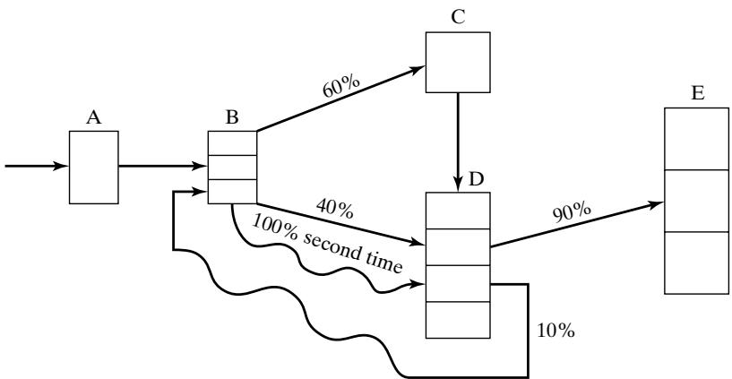 Regular jobs arrive at station A at the rate of one every minutes. Rush jobs arrive every hours and are given a higher priority, except at station C, where they are put on a conveyor and sent through a cleaning and degreasing operation along with all other jobs. For jobs the firs
time through a station, processing and repair times are as follows:
| Station | Number of Machines or Workers | Processing and/or Repair Times (minutes) | Description |
|---|---|---|---|
| A | 1 | Receiving clerk | |
| B | 3 | Disassembly and parts replacement | |
| C | 1 | 20 | Degreaser |
| D | 4 | Reassembly and adjustments | |
| E | 3 | Packing and shipping |
The times listed above hold for all jobs that follow one of the two sequences A B . However, about 10% of the jobs coming out of station D are sent back to B for further work (which takes minutes) and then are sent to D and finally to E. The path of these jobs is as follows:
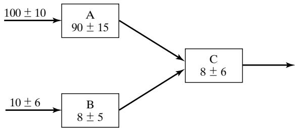
Every 2 hours, beginning 1 hour after opening, the degreasing station C shuts down for routine maintenance, which takes 101 minute. However, this routine maintenance does not begin unti the current widget, if any, has completed its processing. (a) Make three independent replications of the simulation model, where one replication equals an 8-hour simulation run, preceded by a 2-hour initialization run. The three sets of output represent three typical days. The main performance measure of interest is mean response time per job, where a response time is the total time a job spends in the shop. The shop is never empty in the morning, but the model will be empty without the initialization phase. So run the model for a 2-hour initialization period and collect statistics from time 2 hours to time 10 hours. This “warm-up” period will reduce the downward bias in the estimate of mean response time. Note that the 2-hour warm-up is a device to load a simulation model to some more realistic level than empty. From each of the three independen replications, obtain an estimate of mean response time. Also obtain an overall estimate, the sample average of the three estimates.
(b) Management is considering putting one additional worker at the busiest station (A, B, D, or E). Would this significantly improve mean response time? (c) As an alternative to part (b), management is considering replacing machine C with a faster one that processes a widget in only 14 minutes. Would this significantly improve mean response time?
A building-materials firm loads trucks with two payloader tractors. The distribution of truckloading times has been found to be exponential, with a mean loading time of 6 minutes. The truck interarrival time is exponentially distributed with an arrival rate of 16 per hour. The waiting time of a truck and driver is estimated to cost $50 per hour. How much (if any) could the firm save (per 10-hour day) if an overhead hopper system that would fill any truck in a constant time of 2 minutes is installed? (Assume that the present tractors could and would adequately service the conveyors loading the hoppers.)
A milling-machine department has 10 machines. The runtime until failure occurs on a machine is exponentially distributed with a mean of 20 hours. Repair times are uniformly distributed between 3 and 7 hours. Select an appropriate run length and appropriate initial conditions. (a) How many repair people are needed to ensure that the mean number of machines running is greater than eight? (b) If there are two repair people, estimate the number of machines that are either running or being serviced.
Forty people are waiting to pass through a turnstile that takes seconds to traverse. Simulate this system 10 times, each one independent of the others, and determine the range and the average time for all 40 people to traverse.
People borrow Gone with the Wind from the local library and keep it for days. There is only one copy of the book in the library. You are the sixth person on the reservation list (five are ahead of you). Simulate 50 independent cycles of book borrowing to determine the probability that you will receive the book within 100 days.
Jobs arrive every 300 30 seconds to be handled by a process that consists of four operations: OP10 requires seconds, OP20 requires seconds, OP30 require seconds, OP40 requires seconds. Simulate this process until 250 jobs are completed; then combine the four operations of the job into one with the distribution seconds and simulate the process with this distribution. Does the average time in the system change for the two alternatives?
Two types ofjobs arrive to be processed on the same machine. Type 1 jobs arrive every seconds and require seconds for processing. Type 2 jobs arrive every seconds and require seconds for processing. For an 8-hour simulation, what is the average number of jobs waiting to be processed?
Two types ofjobs arrive to be processed on the same machine. Type 1 jobs arrive every seconds and require 35 20 seconds for processing. Type 2 jobs arrive every 100 40 seconds and require 20 15 seconds for processing. Engineering has judged that there is excess capacity on the machine. For a simulation of 8 hours of operation of the system, find X for Type 3 jobs that arrive every seconds and require a time of 30 seconds on the machine so that the average number of jobs waiting to be processed is two or less.
Using spreadsheet software, generate 1000 uniformly distributed random values with mean 10 and spread 2. Plot these values with intervals of width 0.5 between 8 and 12. How close did the simulated set of values come to the expected number in each interval?
Using a spreadsheet, generate 1000 exponentially distributed random values with a mean of 10. What is the maximum of the simulated values? What fraction of the generated values is less than the mean of 10? Plot a histogram of the generated values. [Hint: If you cannot find an exponential generator in the spreadsheet you use, use the formula , where R is a uniformly distributed random number from 0 to 1 and LOG is the natural logarithm.]
There are many “boids” simulations on the internet. Search the internet for two examples of a boids simulation. For each one, find a description of the rules that each boid follows. Compare and contrast the two sets of rules. At a minimum, answer the following questions regarding each model. (a) Are the boids flying in a 2-D or 3-D space? Are they flying in a world with boundary, or without boundary? [Hint: Do they turn at edges or walls? Or do they re-appear on the other side? If so, this implies that two apparent boundaries are glued together and are not really boundaries at all.] Describe the world or universe in which the boids are flying. (b) Does the model have user-adjustable parameters? Such parameters may include the number of boids, the closeness factor (how close one boid must be to other boids before it’s affected by the other’s behavior), speed, and so forth. Make a list of all such parameters. (c) How long does it take for flocking behavior to emerge?
List of Materials Available on www.bcnn.net
Base classes for programming-language based simulations