5 Statistical Models in Simulation
In modeling real-world phenomena, there are few situations where the actions ofthe entities within the system under study can be predicted completely. The world the model builder sees is probabilistic rather than deterministic. There are many causes of variation. The time it takes a repairperson to fix a broken machine is a function of the complexity of the breakdown, whether the repairperson brought the proper replacement parts and tools to the site, whether another repairperson asks for assistance during the course ofthe repair, whether the machine operator receives a lesson in preventive maintenance, and so on. To the model builder, these variations appear to occur by chance and canno be predicted. However, some statistical model might well describe the time to make a repair.
An appropriate model can be developed by sampling the phenomenon of interest. Then, through educated guesses (or using software for the purpose), the model builder would select a known distribution form, make an estimate of the parameter(s) of this distribution, and then test to see how good a fit has been obtained. Through continued efforts in the selection of an appropriate distribution form, a postulated model could be accepted.
Section 1 contains a review of probability terminology and concepts. Some typical applications of statistical models, or distribution forms, are given in Section 2. Then, a number of selected discrete and continuous distributions are discussed in Sections 3 and 4. The selected distributions are those tha describe a wide variety of probabilistic events. Additional discussion about the distribution forms appearing in this chapter, and about distribution forms mentioned but not described, is available from a number of sources [Devore, 1999; Hines and Montgomery, 1990; Law and Kelton, 2000; Papoulis, 1990; Ross, 2002; Walpole and Myers, 2002]. Section 5 describes the Poisson process and its relationship to the exponential distribution. Section 6 discusses empirical distributions.
1 Review of Terminology and Concepts
1.1 Discrete random variables
Let X be a random variable. If the number of possible values of X is finite, or countably infinite, X is called a discrete random variable. The possible values of X may be listed as . In the finite case, the list terminates; in the countably infinite case, the list continues indefinitely.
Example 1
The number of jobs arriving each week at a job shop is observed. The random variable of interest is X, where
The possible values of X are given by the range space of X, which is denoted by . Here Let X be a discrete random variable. With each possible outcome in , a number gives the probability that the random variable equals the value of x . The numbers must satisfy the following two conditions:
a., for all i
The collection of pairs . is called the probability distribution of X, and is called the probability mass function (pmf) of X.
Example 2
Consider the experiment of tossing a single die. Define X as the number of spots on the up face of the die after a toss. Then . Assume the die is loaded so that the probability that a given face lands up is proportional to the number of spots showing. The discrete probability distribution for this random experiment is given by
| 1 | 2 | 3 | 4 | 5 | 6 | |
|---|---|---|---|---|---|---|
| 1/21 | 2/21 | 3/21 | 4/21 | 5/21 | 6/21 |
The conditions stated earlier are satisfied—that is, for and . The distribution is shown graphically in Figure 1.
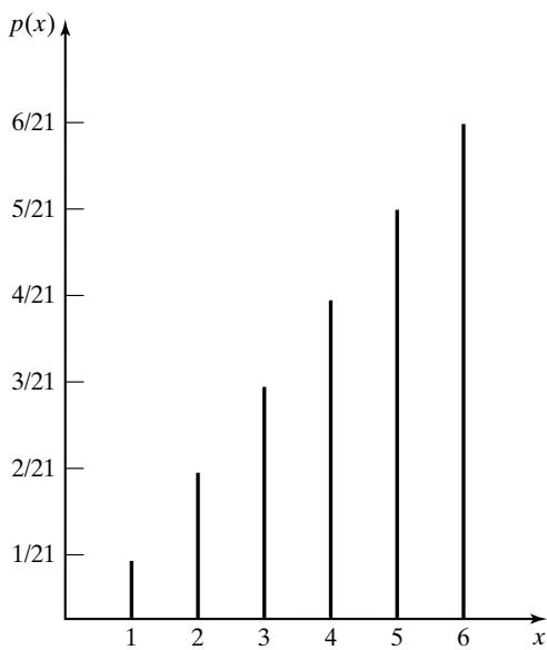 Figure 1 Probability mass function for loaded-die example.
1.2 Continuous random variables
If the range space of the random variable X is an interval or a collection of intervals, X is called a continuous random variable. For a continuous random variable X, the probability that X lies in the interval [a, b] is given by
The function is called the probability density function (pdf) of the random variable X. The pdf satisfies the following conditions:
a. for all x in b. c. if x is not in As a result of Equation (1), for any specified value , because
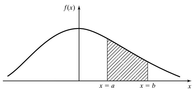 Figure 2 Graphical interpretation of also means that the following equations hold:
The graphical interpretation of Equation (1) is shown in Figure 2. The shaded area represents the probability that X lies in the interval [a, b].
Example 3
The life of a device used to inspect cracks in aircraft wings is given by X, a continuous random variable assuming all values in the range . The pdf of the device’s lifetime, in years, is as follows:
This pdf is shown graphically in Figure 3. The random variable X is said to have an exponentia distribution with mean 2 years.
The probability that the life of the device is between 2 and 3 years is calculated as
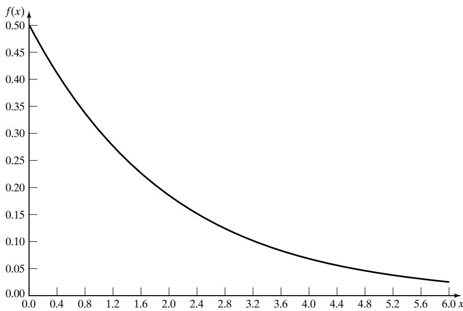 Figure 3 pdf for inspection-device life.
1.3 Cumulative distribution function
The cumulative distribution function (cdf), denoted by , measures the probability that the random variable X assumes a value less than or equal to x, that is,.
If X is discrete, then
If X is continuous, then
Some properties of the cdf are listed here:
a. F is a nondecreasing function. If , then ).
b. lim c. lim All probability questions about X can be answered in terms of the cdf. For example,
For continuous distributions, not only does Equation (5) hold, but also the probabilities in Equation (2) are equal to
Example 4
The die-tossing experiment described in Example 2 has a cdf given as follows:
| x | |||||||
|---|---|---|---|---|---|---|---|
| F(x) | 0 | 1/21 | 3/21 | 6/21 | 10/21 | 15/21 | 21/21 |
where [a,. The cdf for this example is shown graphically in Figure 4.
If X is a discrete random variable with possible values , where , the cdf is a step function. The value of the cdf is constant in the interval and then takes a step, or jump, of size at . Thus, in Example 4,, which is the size of the step when 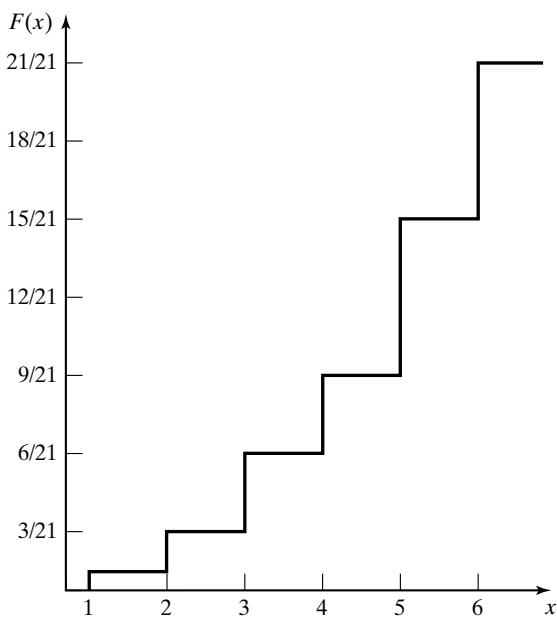 Figure 4 cdf for loaded-die example.
Example 5
The cdf for the device described in Example 3 is given by
The probability that the device will last for less than 2 years is given by
The probability that the life of the device is between 2 and 3 years is calculated as
as found in Example 3.
1.4 Expectation
An important concept in probability theory is that of the expectation of a random variable. If X is a random variable, the expected value of X, denoted by , for discrete and continuous variables, is defined as follows:
and
The expected value E(X) of a random variable X is also referred to as the mean,, or the first moment of X. The quantity , is called the nth moment of X, and is computed as follows:
and
The variance of a random variable X denoted by V(X) or var(X) or , is defined by
A useful identity in computing V(X) is given by
The mean is a measure of the central tendency of a random variable. The variance of X measures the expected value of the squared difference between the random variable and its mean. Thus, the variance,, is a measure of the spread or variation of the possible values of X around the mean . The standard deviation, σ, is defined to be the square root of the variance,. The mean,, and the standard deviation,, are expressed in the same units.
Example 6
The mean and variance of the die-tossing experiment described in Example 2 are computed as follows:
To compute from Equation (10), first compute from Equation (8) as follows:
Thus,
and
Example 7
The mean and variance of the life of the device described in Example 3 are computed as follows:
To compute from Equation (10), first compute ) from Equation (9) as follows:
Thus,
giving
Statistical Models in Simulation
and
With a mean life of 2 years and a standard deviation of 2 years, most analysts would conclude tha actual lifetimes, X, have a fairly large variability.
1.5 The mode
The mode is used in describing several statistical models that appear in this chapter. In the discrete case, the mode is the value of the random variable that occurs most frequently. In the continuous case, the mode is the value at which the pdf is maximized. The mode might not be unique; if the modal value occurs at two values of the random variable, the distribution is said to be bimodal.
2 Useful Statistical Models
Numerous situations arise in the conduct of a simulation where an investigator may choose to introduce probabilistic events. In a queueing system, interarrival and service times are often probabilistic. In an inventory model, the time between demands and the lead times (time between placing and receiving an order) can be probabilistic. In a reliability model, the time to failure could be probabilistic. In each of these instances, the simulation analyst desires to generate random events and to use a known statistical model if the underlying distribution can be found. In the following paragraphs, statistical models appropriate to these application areas will be discussed. Additionally, statistica models useful in the case of limited data are mentioned.
2.1 Queueing systems
In queueing examples, interarrival- and service-time patterns, the times between arrivals and the service times are often probabilistic. However, it is possible to have a constant interarrival time (as in the case of a line moving at a constant speed in the assembly of an automobile), or a constant service time (as in the case of robotized spot welding on the same assembly line). The following example illustrates how probabilistic interarrival times might occur.
Example 8
Mechanics arrive at a centralized tool crib as shown in Table 1. Attendants check in and check out the requested tools to the mechanics. The collection of data begins at 10:00 A.M. and continues unti 20 different interarrival times are recorded. Rather than record the actual time of day, the absolute time from a given origin could have been computed Thus the first mechanic could have arrived at time the second mechanic at time 7:13 (7 minutes, 13 seconds), and so on.
Table 1 Mechanics’ Arrival Data
| Arrival Number | Arrival (hour:minutes::seconds) | Interarrival Time (minutes::seconds) |
|---|---|---|
| 1 | 10:05::03 | — |
| 2 | 10:12::16 | 7::13 |
| 3 | 10:15::48 | 3::32 |
| 4 | 10:24::27 | 8::39 |
| 5 | 10:32::19 | 7::52 |
| 6 | 10:35::43 | 3::24 |
| 7 | 10:39::51 | 4::08 |
| 8 | 10:40::30 | 0::39 |
| 9 | 10:41::17 | 0::47 |
| 10 | 10:44::12 | 2::55 |
| 11 | 10:45::47 | 1::35 |
| 12 | 10:50::47 | 5::00 |
| 13 | 11:00::05 | 9::18 |
| 14 | 11:04::58 | 4::53 |
| 15 | 11:06::12 | 1::14 |
| 16 | 11:11::23 | 5::11 |
| 17 | 11:16::31 | 5::08 |
| 18 | 11:17::18 | 0::47 |
| 19 | 11:21::26 | 4::08 |
| 20 | 11:24::43 | 3::17 |
| 21 | 11:31::19 | 6::36 |
Example 9
Another way of presenting interarrival data is to find the number of arrivals per time period. Here, such arrivals occur over approximately 1.5 hours; it is convenient to look at 10-minute time intervals for the first 20 mechanics. That is, in the first 10-minute time period, one arrival occurred at 10:05::03. In the second time period, two mechanics arrived, and so on. The results are summarized in Table 2. This data could then be plotted in a histogram, as shown in Figure 5.
The distribution of time between arrivals and the distribution of the number of arrivals per time period are important in the simulation of waiting-line systems. “Arrivals” occur in numerous ways; as machine breakdowns, as jobs coming into a job shop, as units being assembled on a line, as orders to a warehouse, as data packets to a computer system, as calls to a call center, and so on.
Service times could be constant or probabilistic. If service times are completely random, the exponential distribution is often used for simulation purposes; however, there are several other possibilities. It could happen that the service times are constant, but some random variability causes fluctuations in either a positive or a negative way. For example, the time it takes for a lathe to traverse a 10-centimeter shaft should always be the same. However, the material could have slight differences in hardness or the tool might wear; either event could cause different processing times. In these cases, the normal distribution might describe the service time.
Table 2 Arrivals in Successive Time Period
| Time Period | Number of Arrivals | Time Period | Number of Arrivals |
|---|---|---|---|
| 1 | 1 | 6 | 1 |
| 2 | 2 | 7 | 3 |
| 3 | 1 | 8 | 3 |
| 4 | 3 | 9 | 2 |
| 5 | 4 | — | — |
A special case occurs when the phenomenon of interest seems to follow the normal probability distribution, but the random variable is restricted to be greater than or less than a certain value. In this case, the truncated normal distribution can be utilized.
The gamma and Weibull distributions are also used to model interarrival and service times. (Actually, the exponential distribution is a special case of both the gamma and the Weibull distributions.) The differences between the exponential, gamma, and Weibull distributions involve the location of the modes of the pdfs and the shapes of their tails for large and small times. The exponential distribution has its mode at the origin, but the gamma and Weibull distributions have their modes at some point that is a function of the parameter values selected. The tail of the gamma distribution is long, like an exponential distribution; the tail of the Weibull distribution can decline more rapidly or less rapidly than that of an exponential distribution. In practice, this means that, if there are more large service times than an exponential distribution can account for, a Weibul distribution might provide a better model of these service times.
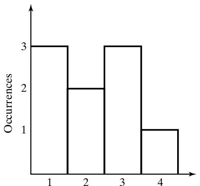 Number of arrivals in 10-minute period
Figure 5 Histogram of arrivals per time period.
2.2 Inventory and supply-chain systems
In realistic inventory and supply-chain systems, there are at least three random variables: (1) the number ofunits demanded per order or per time period, (2) the time between demands, and (3) the lead time. (The lead time is defined as the time between the placing of an order for stocking the inventory system and the receipt of that order.) In very simple mathematical models of inventory systems, demand is a constant over time, and lead time is zero, or a constant. However, in most real-world cases, and, hence, in simulation models, demand occurs randomly in time, and the number of units demanded each time a demand occurs is also random, as illustrated by Figure 6.
Distributional assumptions for demand and lead time in inventory theory texts are usually based on mathematical tractability, but those assumptions could be invalid in a realistic context. In practice, the lead-time distribution can often be fitted fairly well by a gamma distribution [Hadley and Whitin, 1963]. Unlike analytic models, simulation models can accommodate whatever assumptions appear most reasonable.
The geometric, Poisson, and negative binomial distributions provide a range of distribution shapes that satisfy a variety of demand patterns. The geometric distribution, which is a special case of the negative binomial, has its mode at unity, given that at least one demand has occurred. If demand data are characterized by a long tail, the negative binomial distribution might be appropriate. The Poisson distribution is often used to model demand because it is simple, it is extensively tabulated, and it is well known. The tail of the Poisson distribution is generally shorter than that of the negative binomial, which means that fewer large demands will occur if a Poisson model is used than if a negative binomial distribution is used (assuming that both models have the same mean demand).
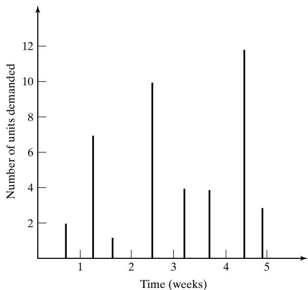 Figure 6 Random demands in time.
2.3 Reliability and maintainability
Time to failure has been modeled with numerous distributions, including the exponential, gamma, and Weilbull. If only random failures occur, the time-to-failure distribution may be modeled as exponential. The gamma distribution arises from modeling standby redundancy, where each component has an exponential time to failure. The Weibull distribution has been extensively used to represent time to failure, and its nature is such that it can be made to approximate many observed phenomena [Hines and Montgomery, 1990]. When there are a number of components in a system and failure is due to the most serious of a large number of defects, or possible defects, the Weibull distribution seems to do particularly well as a model. In situations where most failures are due to wear, the normal distribution might very well be appropriate [Hines and Montgomery, 1990]. The lognormal distribution has been found to be applicable in describing time to failure for some types of components.
2.4 Limited data
In many instances, simulations begin before data collection has been completed. There are three distributions that have application to incomplete or limited data. These are the uniform, triangular, and beta distributions. The uniform distribution can be used when an interarrival or service time is known to be random, but no information is immediately available about the distribution [Gordon, 1975]. However, there are those who do not favor using the uniform distribution, calling it the “distribution of maximum ignorance” because it is not necessary to specify more than the continuous interval in which the random variable may occur. The triangular distribution can be used when assumptions are made about the minimum, maximum, and modal values of the random variable. Finally, the beta distribution provides a variety of distributional forms on the unit interval, ones that, with appropriate modification, can be shifted to any desired interval. The uniform distribution is a special case of the beta distribution. Pegden, Shannon, and Sadowski [1995] discuss the subject of limited data in some detail.
2.5 Other distributions
Several other distributions may be useful in discrete-system simulation. The Bernoulli and binomia distributions are two discrete distributions which might describe phenomena of interest. The hyperexponential distribution is similar to the exponential distribution, but its greater variability might make it useful in certain instances.
3 Discrete Distributions
Discrete random variables are used to describe random phenomena in which only integer values can occur. Numerous examples were given in Section 2—for example, demands for inventory items. Four distributions are described in the following subsections.
3.1 Bernoulli trials and the Bernoulli distribution
Consider an experiment consisting of n trials, each of which can be a success or a failure. Let if the jth experiment resulted in a success, and let if the jth experiment resulted in a failure.
The n Bernoulli trials are called a Bernoulli process if the trials are independent, each trial has only two possible outcomes (success or failure), and the probability of a success remains constant from trial to trial. Thus,
and
For one trial, the distribution given in Equation (11) is called the Bernoulli distribution. The mean and variance of are calculated as follows:
and
3.2 Binomial distribution
The random variable X that denotes the number of successes in n Bernoulli trials has a binomia distribution given by , where
Equation (12) is motivated by computing the probability ofa particular outcome with all the successes, each denoted by S, occurring in the first x trials, followed by the failures, each denoted by an F—that is,
where . There are
outcomes having the required number of and . Therefore, Equation (12) results. An easy approach to calculating the mean and variance of the binomial distribution is to consider X as a sum of n independent Bernoulli random variables, each with mean and variance . Then,
and the mean, E(X), is given by
and the variance V(X) is given by
Example 10
A production process manufactures computer chips on the average at nonconforming. Every day, a random sample of size 50 is taken from the process. If the sample contains more than two nonconforming chips, the process will be stopped. Compute the probability that the process is stopped by the sampling scheme.
Consider the sampling process as Bernoulli trials, each with ; then the total number of nonconforming chips in the sample, X, would have a binomial distribution given by
It is much easier to compute the right-hand side of the following identity to compute the probability that more than two nonconforming chips are found in a sample:
The probability is calculated from
Thus, the probability that the production process is stopped on any day, based on the sampling process, is approximately 0.08. The mean number of nonconforming chips in a random sample of size 50 is given by
and the variance is given by
The cdf for the binomial distribution has been tabulated by Banks and Heikes [1984] and others. The tables decrease the effort considerably for computing probabilities such as ). Under certain conditions on n and both the Poisson distribution and the normal distribution may be used to approximate the binomial distribution [Hines and Montgomery, 1990].
3.3 Geometric and Negative Binomial distributions
The geometric distribution is related to a sequence of Bernoulli trials; the random variable of interest, X, is defined to be the number of trials to achieve the first success. The distribution of X is given by
The event occurs when there are failures followed by a success. Each of the failures has an associated probability of , and each success has probability Thus,
The mean and variance are given by
and
More generally, the negative binomial distribution is the distribution of the number of trials unti the kth success, for has a negative binomial distribution with parameter and k, then the distribution of Y is given by
Because we can think of the negative binomial random variable Y as the sum of independen geometric random variables, it is easy to see that and
Example 11
Forty percent of the assembled ink-jet printers are rejected at the inspection station. Find the probability that the first acceptable ink-jet printer is the third one inspected. Considering each inspection as a Bernoulli trial with and yields
Thus, in only about 10% of the cases is the first acceptable printer the third one from any arbitrary starting point. To determine the probability that the third printer inspected is the second acceptable printer, we use the negative binomial distribution Equation (18),
3.4 Poisson distribution
The Poisson distribution describes many random processes quite well and is mathematically quite simple. The Poisson distribution was introduced in 1837 by S. D. Poisson in a book concerning criminal and civil justice matters. (The title of this rather old text is Recherches sur la probabilit´e desjugements en mati`ere criminelle et en mati`ere civile. Evidently, the rumor handed down through generations of probability theory professors concerning the origin of the Poisson distribution is jus not true. Rumor has it that the Poisson distribution was first used to model deaths from the kicks o horses in the Prussian Army.)
The Poisson probability mass function is given by
where α. One of the important properties of the Poisson distribution is that the mean and variance are both equal to α, that is,
The cumulative distribution function is given by
The pmf and cdf for a Poisson distribution with are shown in Figure 7. A tabulation of the cd is given in Table A.4 in the Appendix.
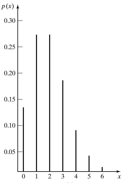 (a)
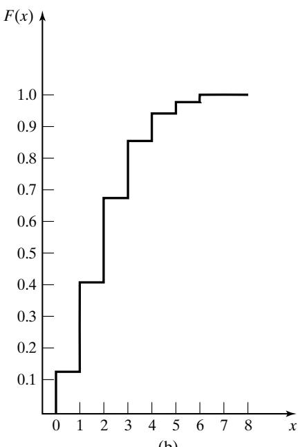 (b)
Figure 7 Poisson pmf and cdf.
Example 12
A computer repair person is “beeped” each time there is a call for service. The number of beeps per hour is known to occur in accordance with a Poisson distribution with a mean of per hour. The probability of three beeps in the next hour is given by Equation (19) with , as follows:
This same result can be read from the left side of Figure 7 or from Table A.4 by computing
Example 13
In Example 12, find the probability of two or more beeps in a 1-hour period.
The cumulative probability,, can be read from the right side of Figure 7 or from Table A.4.
Example 14
The lead-time demand in an inventory system is the accumulation of demand for an item from the point at which an order is placed until the order is received—that
where is the lead-time demand, is the demand during the ith time period, and T is the number of time periods during the lead time. Both and may be random variables.
An inventory manager desires that the probability of a stockout not exceed a certain fraction during the lead time. For example, it may be stated that the probability of a shortage during the lead time not exceed 5%.
If the lead-time demand is Poisson distributed, the determination of the reorder point is greatly facilitated. The reorder point is the level of inventory at which a new order is placed.
Assume that the lead-time demand is Poisson distributed with a mean of units and that 95% protection from a stockout is desired. Thus, it is desired to find the smallest value of x such that the probability that the lead-time demand not exceed x is greater than or equal to 0.95. Using Equation (20) requires finding the smallest x such that
The desired result occurs at , which can be found by using Table A.4 or by computation of
4 Continuous Distributions
Continuous random variables can be used to describe random phenomena in which the variable o interest can take on any value in some interval—for example, the time to failure or the length of a rod. Nine distributions are described in the following subsections.
4.1 Uniform distribution
A random variable X is uniformly distributed on the interval [a, b] if its pdf is given by
The cdf is given by
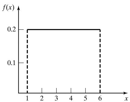
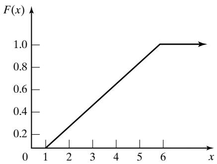 Figure 8 pdf and cdf for uniform distribution.
Note that
is proportional to the length of the interval, for all and satisfying The mean and variance of the distribution are given by
and
The pdf and cdf when and are shown in Figure 8.
The uniform distribution plays a vital role in simulation. Random numbers, uniformly distributed between 0 and 1, provide the means to generate random events. Numerous methods for generating uniformly distributed random numbers have been devised. Uniformly distributed random numbers are then used to generate samples of random variates from all other distributions.
Example 15
A simulation of a warehouse operation is being developed. About every 3 minutes, a call comes for a forklift truck operator to proceed to a certain location. An initial assumption is made that the time between calls (arrivals) is uniformly distributed with a mean of 3 minutes. By Equation (25), the uniform distribution with a mean of 3 and the greatest possible variability would have parameter values of and minutes. With very limited data (such as a mean of approximately 3 minutes) plus the knowledge that the quantity of interest is variable in a random fashion, the uniform distribution with greatest variance can be assumed, at least until more data are available.
Example 16
A bus arrives every 20 minutes at a specified stop beginning at 6:40 A.M. and continuing unti 8:40 A.M. A certain passenger does not know the schedule, but arrives randomly (uniformly distributed) between 7:00 A.M. and 7:30 A.M. every morning. What is the probability that the passenger waits more than 5 minutes for a bus?
The passenger has to wait more than 5 minutes only if the arrival time is between 7:00 A.M. and 7:15 A.M. or between 7:20 A.M. and 7:30 A.M. If X is a random variable that denotes the number of minutes past 7:00 A.M. that the passenger arrives, the desired probability is
Now, X is a uniform random variable on (0, 30). Therefore, the desired probability is given by
4.2 Exponential distribution
A random variable X is said to be exponentially distributed with parameter if its pdf is given by
The density function is shown in Figures 9 and 3. Figure 9 also shows the cdf.
The exponential distribution has been used to model interarrival times when arrivals are completely random and to model service times that are highly variable. In these instances, λ is a rate: arrivals per hour or services per minute. The exponential distribution has also been used to model the lifetime of a component that fails catastrophically (instantaneously), such as a light bulb; then λ is the failure rate.
Several different exponential pdfs are shown in Figure 10. The value of the intercept on the vertical axis is always equal to the value of λ. Note also that all pdfs eventually intersect. (Why?)
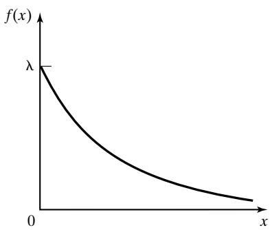
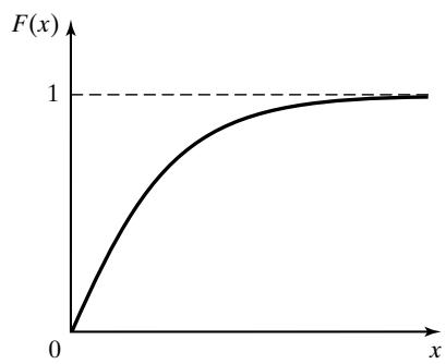 Figure 9 Exponential density function and cumulative distribution function.
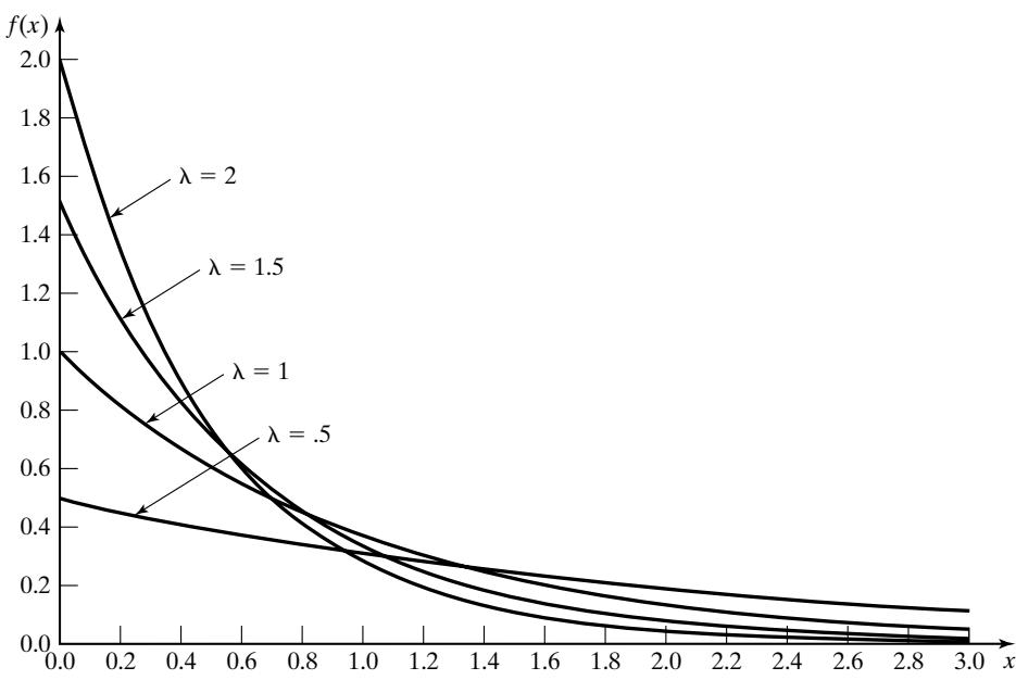 Figure 10 pdfs for several exponential distributions.
The exponential distribution has mean and variance given by
Thus, the mean and standard deviation are equal. The cdf can be exhibited by integrating Equation (26) to obtain
Example 17
Suppose that the life of an industrial lamp, in thousands of hours, is exponentially distributed with failure rate (one failure every 3000 hours, on the average). The probability that the lamp will last longer than its mean life, 3000 hours, is given by Equation (28) is used to compute F(3), obtaining
Regardless of the value of , this result will always be the same! That is, the probability that an exponential random variable is greater than its mean is 0.368, for any value o The probability that the industrial lamp will last between 2000 and 3000 hours is computed as
Again, from the cdf given by Equation (28),
One of the most important properties of the exponential distribution is that it is “memoryless,” which means that, for all and
Let X represent the life of a component (a battery, light bulb, computer chip, laser, etc.) and assume that X is exponentially distributed. Equation (29) states that the probability that the component lives for at least hours, given that it has survived s hours, is the same as the initial probability that it lives for at least t hours. If the component is alive at time s (if , then the distribution of the remaining amount of time that it survives, namely , is the same as the original distribution of a new component. That is, the component does not “remember” that it has already been in use for a time s. A used component is as good as new.
That Equation (29) holds is shown by examining the conditional probability
Equation (28) can be used to determine the numerator and denominator of Equation (30), yielding
Example 18
Find the probability that the industrial lamp in Example 17 will last for another 1000 hours, given that it is operating after 2500 hours. This determination can be found using Equations (29) and (28), as follows:
Example 18 illustrates the memoryless property—namely, that a used component that follows an exponential distribution is as good as a new component. The probability that a new component will have a life greater than 1000 hours is also equal to 0.717. Stated in general, suppose that a component which has a lifetime that follows the exponential distribution with parameter λ is observed and found to be operating at an arbitrary time. Then, the distribution of the remaining lifetime is also exponential with parameter λ. The exponential distribution is the only continuous distribution that has the memoryless property. (The geometric distribution is the only discrete distribution that possesses the memoryless property.)
4.3 Gamma distribution
A function used in defining the gamma distribution is the gamma function, which is defined for al as
By integrating Equation (31) by parts, it can be shown that
If is an integer, then, by using and applying Equation (32), it can be seen that
The gamma function can be thought of as a generalization of the factorial notion to all positive numbers, not just integers.
A random variable X is gamma distributed with parameters and θ if its pdf is given by
is called the shape parameter, and is called the scale parameter. Several gamma distributions for and various values of are shown in Figure 11.
The mean and variance of the gamma distribution are given by
and
The cdf of X is given by
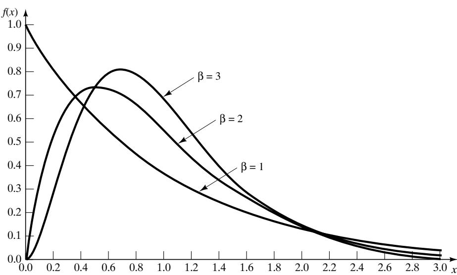 Figure 11 pdfs for several gamma distributions with When is an integer, the gamma distribution is related to the exponential distribution in the following manner: If the random variable X is the sum of independent, exponentially distributed random variables, each with parameter , then X has a gamma distribution with parameters and θ. Thus, i
where the pdf of is given by
and the are mutually independent, then X has the pdf given in Equation (34). Note that, when , an exponential distribution results. This result follows from Equation (38) or from letting in Equation (34).
4.4 Erlang distribution
The pdf given by Equation (34) is often referred to as the Erlang distribution of order (or number of phases) k when an integer. Erlang was a Danish telephone engineer who was an early developer of queueing theory. The Erlang distribution could arise in the following context: Consider a series of k stations that must be passed through in order to complete the servicing of a customer. An additional customer cannot enter the first station until the customer in process has negotiated all the stations. Each station has an exponential distribution of service time with parameter kθ. Equations (35) and (36), which state the mean and variance of a gamma distribution, are valid regardless of the value of . However, when an integer, Equation (38) may be used to derive the mean of the distribution in a fairly straightforward manner. The expected value of the sum of random variables is the sum of the expected value of each random variable. Thus,
The expected value of each of the exponentially distributed is given by . Thus,
If the random variables are independent, the variance of their sum is the sum of the variances, or
When , a positive integer, the cdf given by Equation (37) may be integrated by parts, giving
which is the sum of Poisson terms with mean . Tables of the cumulative Poisson distribution may be used to evaluate the cdf when the shape parameter is an integer.
Example 19
A college professor of electrical engineering is leaving home for the summer, but would like to have a light burning at all times to discourage burglars. The professor rigs up a device that will hold two light bulbs. The device will switch the current to the second bulb if the first bulb fails. The box in which the light bulbs are packaged says, “Average life 1000 hours, exponentially distributed.” The professor will be gone 90 days (2160 hours). What is the probability that a light will be burning when the summer is over and the professor returns?
The probability that the system will operate at least x hours is called the reliability function :
In this case, the total system lifetime is given by Equation (38) with bulbs and per hour, so per hour. Thus, can be determined from Equation (39) as follows:
Therefore, the chances are about 36% that a light will be burning when the professor returns.
Example 20
A medical examination is given in three stages by a physician. Each stage is exponentially distributed with a mean service time of 20 minutes. Find the probability that the exam will take 50 minutes or less. Also, compute the expected length of the exam. In this case, stages and , so that per minute. Thus, can be calculated from Equation (39) as follows:
The cumulative Poisson distribution, shown in Table A.4, can be used to calculate that
The probability is 0.457 that the exam will take 50 minutes or less. The expected length of the exam is found from Equation (35):
In addition, the variance of X is minutes^2—incidentally, the mode of the Erlang distribution is given by
Thus, the modal value in this example is
4.5 Normal distribution
A random variable X with mean and variance has a normal distribution if it has the pdf
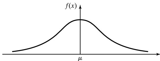 Figure 12 pdf of the normal distribution.
The normal distribution is used so often that the notation ) has been adopted by many authors to indicate that the random variable X is normally distributed with mean and variance The normal pdf is shown in Figure 12.
Some of the special properties of the normal distribution are listed here:
a. lim and lim the value off(x) approaches zero as x approaches negative infinity and, similarly, as x approaches positive infinity.
b.; the pdf is symmetric about .
c. The maximum value of the pdf occurs at the mean and mode are equal.
The cdf for the normal distribution is given by
It is not possible to evaluate Equation (42) in closed form. Numerical methods could be used, but it appears that it would be necessary to evaluate the integral for each pair . However, a transformation of variables,, allows the evaluation to be independent of and . If , let to obtain
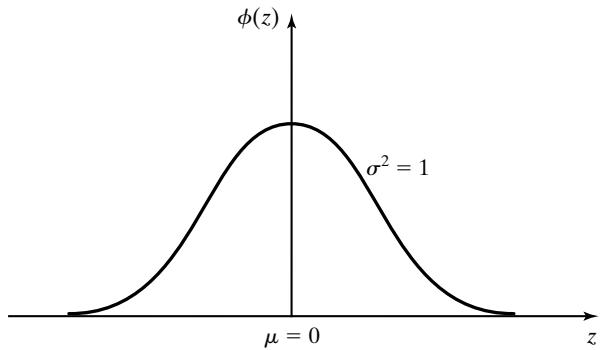 Figure 13 pdf of the standard normal distribution.
The pdf
is the pdf of a normal distribution with mean 0 and variance 1. Thus, and it is said tha has a standard normal distribution. The standard normal distribution is shown in Figure 13. The cdf for the standard normal distribution is given by
Equation (45) has been widely tabulated. The probabilities for are given in Table A.3. Several examples are now given that indicate how Equation (43) and Table A.3 are used.
Example 21
Suppose that it is known that . Compute ). Using Equation (43), we get
from Table A.3. The intuitive interpretation is shown in Figure 14. Figure shows the pdf of with the specific value,, marked. The shaded portion is the desired probability. Figure 14(b) shows the standard normal distribution o ) with the value 2 marked; is 2σ (where greater than the mean. It is helpful to make both sketches such as those in Figure 14 to avoid confusion in figuring out required probabilities.
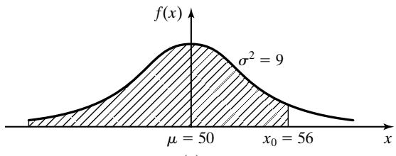 (a)
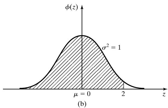 Figure 14 Transforming to the standard normal distribution.
Example 22
The time in hours required to load an ocean-going vessel, X, is distributed as . The probability that the vessel will be loaded in less than 10 hours is given by , where
The value of is looked up in Table A.3 by using the symmetry property of the normal distribution. Note that . The complement of 0.8413, or 0.1587, is contained in the tail, the shaded portion of the standard normal distribution shown in Figure 15(a). In Figure 15(b), the symmetry property is used to work out the shaded region to be [From this logic, it can be seen that and . In general, The probability that 12 or more hours will be required to load the ship can also be discovered by inspection, by using the symmetry property ofthe normal pdfand the mean as shown by Figure 16. The shaded portion of Figure 16(a) shows the problem as originally stated [i.e., evaluate ]. Now,. The standardized normal in Figure 16(b) is used to evaluate . Thus,. (The shaded portions in both Figure 16(a) and (b) contain 0.50 of the area under the normal pdf.)
(a)
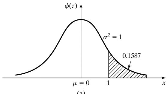
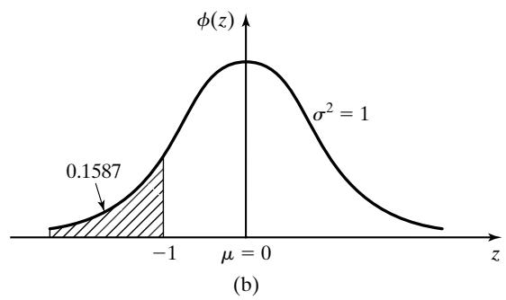 Figure 15 Using the symmetry property of the normal distribution.
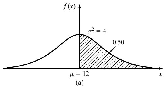
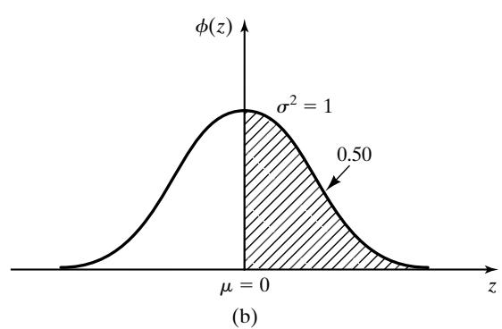 Figure 16 Evaluation of probability by inspection.
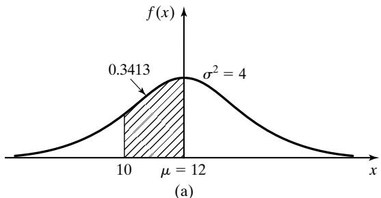
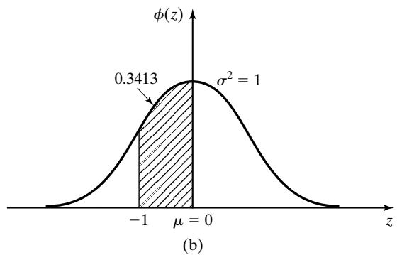 Figure 17 Transformation to standard normal for vessel-loading problem.
The probability that between 10 and 12 hours will be required to load a ship is given by
using earlier results presented in this example. The desired area is shown in the shaded portion of Figure 17(a). The equivalent problem shown in terms of the standardized normal distribution is shown in Figure 17(b). The probability statement is 0.3413, from Table A.3.
Example 23
The time to pass through a queue to begin self-service at a cafeteria has been found to be The probability that an arriving customer waits between 14 and 17 minutes is computed as follows:
The shaded area shown in Figure 18(a) represents the probability . The shaded area shown in Figure 18(b) represents the equivalent probability,), for the standardized normal distribution. From Table A.3,. Now,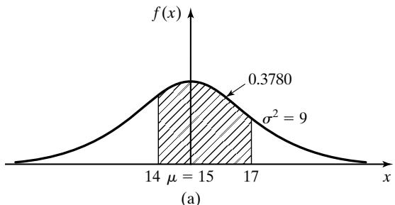
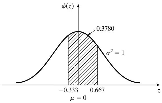 (b)
Figure 18 Transformation to standard normal for cafeteria problem.. Thus,. The probability is 0.3780 that the customer will pass through the queue in a time between 14 and 17 minutes.
Example 24
Lead-time demand, X, for an item is approximated by a normal distribution having mean 25 and variance 9. It is desired to compute the value for lead time that will be exceeded only 5% of the time. Thus, the problem is to find such that , as shown by the shaded area in Figure 19(a). The equivalent problem is shown as the shaded area in Figure 19(b). Now,
or, equivalently,
From Table A.3, it can be seen that (1.645) 0.95. Thus, can be found by solving
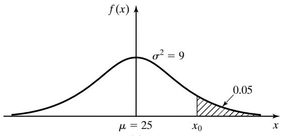 (a)
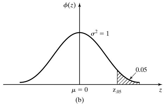 Figure 19 Finding for lead-time-demand problem.
Therefore, in only 5% of the cases will demand during lead time exceed available inventory if an order to purchase is made when the stock level reaches 30.
4.6 Weibull distribution
The random variable X has a Weibull distribution if its pdf has the form
The three parameters of the Weibull distribution are ν, which is the location parameter; α, which is the scale parameter; and , which is the shape parameter. When , the Weibull pdf becomes
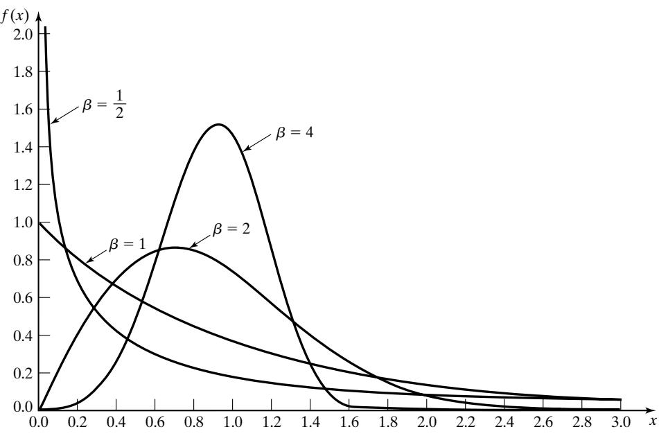 Figure ^20 Weibull pdfs for ν = 0; α = 1; β = ^1 , 1, 2, 4.
Figure 20 shows several Weibull densities when and . When , the Weibul distribution is reduced to
which is an exponential distribution with parameter The mean and variance of the Weibull distribution are given by the following expressions:
where is defined by Equation (31). Thus, the location parameter ν has no effect on the variance; however, the mean is increased or decreased by ν. The cdf of the Weibull distribution is given by
Example 25
The time to failure for a component is known to have a Weibull distribution with and . The mean time to failure is given by Equation (48) as
The probability that a unit fails before 2000 hours is computed from Equation (50) as
Example 26
The time it takes for an aircraft to land and clear the runway at a major international airport has a Weibull distribution with minutes, minutes, and . Find the probability that an incoming airplane will take more than 1.5 minutes to land and clear the runway. In this case is computed as follows:
Therefore, the probability that an aircraft will require more than 1.5 minutes to land and clear the runway is 0.135.
4.7 Triangular distribution
A random variable X has a triangular distribution if its pdf is given by
where . The mode occurs at . A triangular pdf is shown in Figure 21. The parameters can be related to other measures, such as the mean and the mode, as follows:
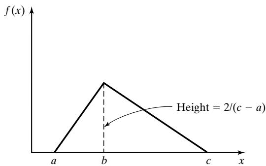 Figure 21 pdf of the triangular distribution.
From Equation (52) the mode can be determined as
Because
The mode is used more often than the mean to characterize the triangular distribution. As is shown in Figure 21, its height is above the x axis. The variance,, of the triangular distribution is left as an exercise for the student. The cdf for the triangular distribution is given by
Example 27
The central processing unit requirements, for programs that will execute, have a triangular distribution with milliseconds, milliseconds, and milliseconds. Find the probability that the CPU requirement for a random program is 2.5 milliseconds or less. The value of F(2.5) is from the portion of the cdf in the interval [0.05, 1.1] plus that portion in the interval [1.1, 2.5]. By using Equation (54), both portions can be addressed at one time, to yield
Thus, the probability is 0.541 that the CPU requirement is 2.5 milliseconds or less.
Example 28
An electronic sensor evaluates the quality of memory chips, rejecting those that fail. Upon demand, the sensor will give the minimum and maximum number of rejects during each hour of production over the past 24 hours. The mean is also given. Without further information, the quality contro department has assumed that the number of rejected chips can be approximated by a triangular distribution. The current dump of data indicates that the minimum number of rejected chips during any hour was 0, the maximum was 10, and the mean was 4. Given that , and the value of b can be found from Equation (53):
The height of the mode is . Thus, Figure 22 can be drawn.
The median is the point at which 0.5 of the area is to the left and 0.5 is to the right. The median in this example is 3.7, also shown on Figure 22. Finding the median of the triangular distribution requires an initial location of the value to the left or to the right of the mode. The area to the left of the mode is computed from Equation (54) as
Thus, the median is between b and c. Setting in Equation (54) and solving for x median yields
with
This example clearly shows that the mean, mode, and median are not necessarily equal.
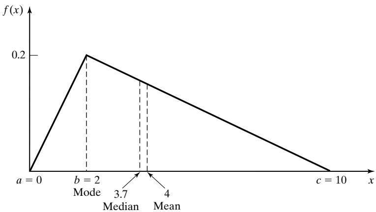 Figure 22 Mode, median, and mean for triangular distribution.
4.8 Lognormal distribution
A random variable X has a lognormal distribution if its pdf is given by
where . The mean and variance of a lognormal random variable are
Three lognormal pdfs, all having mean 1, but variances , 1, and 2, are shown in Figure 23.
Notice that the parameters and are not the mean and variance of the lognormal. These parameters come from the fact that when Y has a ) distribution then has a lognorma distribution with parameters and . If the mean and variance of the lognormal are known to be and , respectively, then the parameters and are given by
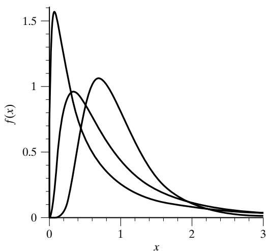 Figure 23 pdf of the lognormal distribution.
Example 29
The rate of return on a volatile investment is modeled as having a lognormal distribution with mean 20% and standard deviation 5%. Compute the parameters for the lognormal distribution. From the information given, we have and . Thus, from Equations (58) and (59),
4.9 Beta distribution
A random variable X is beta distributed with parameters and if its pdf is given by
where . The cdf of the beta does not have a closed form, in general.
The beta distribution is very flexible and has a finite range from 0 to 1, as shown in Figure 24. In practice, we often need a beta distribution defined on a different range, say , with , rather than (0, 1). This is easily accomplished by defining a new random variable
The mean and variance of Y are given by
and
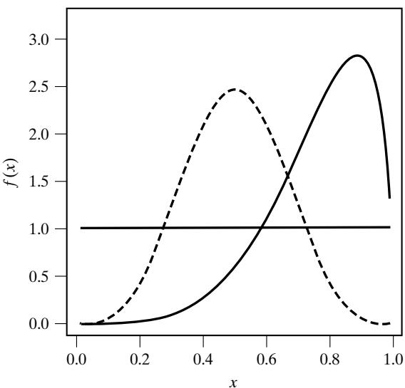 Figure 24 pdf for several beta distributions.
5 Poisson Process
Consider random events such as the arrival ofjobs at a job shop, the arrival of e-mail to a mail server, the arrival of boats to a dock, the arrival of calls to a call center, the breakdown of machines in a large factory, and so on. These events may be described by a counting function defined for all . This counting function will represent the number of events that occurred in [0, t]. Time zero is the point at which the observation began, regardless of whether an arrival occurred at that instant. For each interval , the value is an observation of a random variable where the only possible values that can be assumed by N(t) are the integers The counting process,, is said to be a Poisson process with mean rate λ if the following assumptions are fulfilled:
a. Arrivals occur one at a time.
b. has stationary increments: The distribution of the number of arrivals between t and depends only on the length of the interval s, not on the starting point t. Thus, arrivals are completely at random without rush or slack periods.
c. has independent increments: The number of arrivals during nonoverlapping time intervals are independent random variables. Thus, a large or small number of arrivals in one time interval has no effect on the number of arrivals in subsequent time intervals. Future arrivals occur completely at random, independent of the number of arrivals in past time intervals.
If arrivals occur according to a Poisson process, meeting the three preceding assumptions, it can be shown that the probability that is equal to n is given by
Comparing Equation (63) to Equation (19), it can be seen that has the Poisson distribution with parameter . Thus, its mean and variance are given by
For any times s and t such that the assumption of stationary increments implies that the random variable , representing the number of arrivals in the interval from s to t, is also Poisson-distributed with mean . Thus,
and
Now, consider the time at which arrivals occur in a Poisson process. Let the first arrival occur at time , the second occur at time , and so on, as shown in Figure 25.
Thus,. are successive interarrival times. The first arrival occurs after time t if and only if there are no arrivals in the interval [0, t], so it is seen that
and, therefore,
the last equality following from Equation (63). Thus, the probability that the first arrival will occur in [0, t] is given by
which is the cdf for an exponential distribution with parameter λ. Hence, is distributed exponentially with mean . It can also be shown that all interarrival times, are
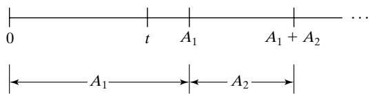 Figure 25 Arrival process.
exponentially distributed and independent with mean . As an alternative definition of a Poisson process, it can be shown that, if interarrival times are distributed exponentially and independently, then the number of arrivals by time t, say , meets the three previously mentioned assumptions and, therefore, is a Poisson process.
Recall that the exponential distribution is memoryless—that is, the probability of a future arriva in a time interval of length s is independent of the time of the last arrival. The probability of the arrival depends only on the length of the time interval s. Thus, the memoryless property is related to the properties of independent and stationary increments of the Poisson process.
Additional readings concerning the Poisson process may be obtained from many sources, including Parzen [1999], Feller [1968], and Ross [2002].
Example 30
The jobs at a machine shop arrive according to a Poisson process with a mean of jobs per hour. Therefore, the interarrival times are distributed exponentially, with the expected time between arrivals being hour.
5.1 Properties of a Poisson Process
Several properties of the Poisson process, discussed by Ross [2002] and others, are useful in discretesystem simulation. The first ofthese properties concerns random splitting. Consider a Poisson process having rate λ, as represented by the left side of Figure 26.
Suppose that, each time an event occurs, it is classified as either a type I or a type II event. Suppose further that each event is classified as a type I event with probability and type II event with probability , independently of all other events.
Let and be random variables that denote, respectively, the number of type I and type II events occurring in [0, t]. Note that ). It can be shown that and are both Poisson processes having rates and , as shown in Figure 26. Furthermore, it can be shown that the two processes are independent.
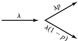 Figure 26 Random splitting.
Example 31: Random Splitting
Suppose thatjobs arrive at a shop in accordance with a Poisson process having rate λ. Suppose further that each arrival is marked “high priority” with probability 1/3 and “low priority” with probability 2/3. Then a type I event would correspond to a high-priority arrival and a type II event would correspond to a low-priority arrival. If and are as just defined, both variables follow the Poisson process, with rates and , respectively.
Example 32
The rate in Example 31 is per hour. The probability that no high-priority jobs will arrive in a 2-hour period is given by the Poisson distribution with parameter . Thus,
Now, consider the opposite situation from random splitting, namely the pooling of two arrival streams. The process of interest is illustrated in Figure 27. It can be shown that, if are random variables representing independent Poisson processes with rates , for and 2, then is a Poisson process with rate 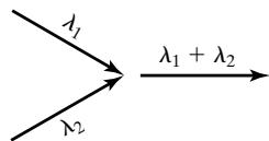 Figure 27 Pooled process.
Example 33: Pooled Process
A Poisson arrival stream with arrivals per hour is combined (or pooled) with a Poisson arrival stream with arrivals per hour. The combined process is a Poisson process with arrivals per hour.
5.2 Nonstationary Poisson Process
If we keep the Poisson Assumptions 1 and 3 (Section 5), but drop Assumption 2 (stationary increments) then we have a nonstationary Poisson process (NSPP), which is characterized by , the arrival rate at time t. The NSPP is useful for situations in which the arrival rate varies during the period of interest, including meal times for restaurants, phone calls during business hours, and orders for pizza delivery around 6 P.M.
The key to working with an NSPP is the expected number of arrivals by time t, denoted by
To be useful as an arrival-rate function, λ(t) must be nonnegative and integrable. For a stationary Poisson process with rate λ we have , as expected.
Let . be the arrival times of stationary Poisson process with , and let . be the arrival times for an NSPP with arrival rate ). The fundamental relationship for working with NSPPs is the following:
In other words, an NSPP can be transformed into a stationary Poisson process with arrival rate 1, and a stationary Poisson process with arrival rate 1 can be transformed into an NSPP with rate λ(t), and the transformation in both cases is related to
Example 34
Suppose that arrivals to a post office occur at a rate of 2 per minute from 8 A.M. until 12 P.M., then drop to 1 every 2 minutes until the day ends at 4 P.M. What is the probability distribution of the number of arrivals between 11 A.M. and 2 P.M?
Let time correspond to 8 A.M. Then this situation could be modeled as an NSPP with rate function
The expected number of arrivals by time t is therefore
Notice that computing the expected number of arrivals for 4 requires that the integration be done in two parts:
Since 2 P.M. and 11 A.M. correspond to times 6 and 3, respectively, we have
where is a stationary Poisson process with arrival rate 1.
6 Empirical Distributions
An empirical distribution, which may be either discrete or continuous in form, is a distribution whose parameters are the observed values in a sample of data. This is in contrast to parametric distribution families (such as the exponential, normal, or Poisson), which are characterized by specifying a smal number of parameters such as the mean and variance. An empirical distribution may be used when i is impossible or unnecessary to establish that a random variable has any particular parametric distribution. One advantage of an empirical distribution is that nothing is assumed beyond the observed values in the sample; however, this is also a disadvantage because the sample might not cover the entire range of possible values.
Example 35: Discrete
Customers at a local restaurant arrive at lunchtime in groups of one to eight people. The number of people per party in the last 300 groups has been observed; the results are summarized in Table 3. The relative frequencies appear in Table 3 and again in Figure 28, which provides a histogram of the data that were gathered. Figure 29 provides a cdf of the data. The cdf in Figure 29 is called the empirica distribution of the given data.
Table 3 Arrivals per Party Distribution
| Arrivals per Party | Frequency | Relative Frequency | Cumulative Relative Frequency |
|---|---|---|---|
| 1 | 30 | 0.10 | 0.10 |
| 2 | 110 | 0.37 | 0.47 |
| 3 | 45 | 0.15 | 0.62 |
| 4 | 71 | 0.24 | 0.86 |
| 5 | 12 | 0.04 | 0.90 |
| 6 | 13 | 0.04 | 0.94 |
| 7 | 7 | 0.02 | 0.96 |
| 8 | 12 | 0.04 | 1.00 |
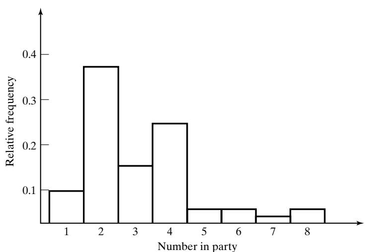 Figure 28 Histogram of party size.
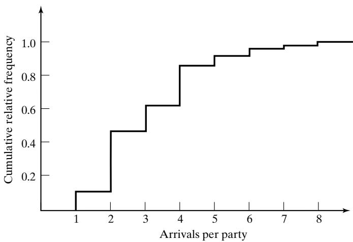 Figure 29 Empirical cdf of party size.
Example 36: Continuous
The time required to repair a conveyor system that has suffered a failure has been collected for the last 100 instances; the results are shown in Table 4. There were 21 instances in which the repair took between 0 and 0.5 hour, and so on. The empirical cdf is shown in Figure 30. A piecewise linear curve is formed by the connection of the points of the form [x, F(x)]. The points are connected by a straigh line. The first connected pair is (0, 0) and (0.5, 0.21); then the points (0.5, 0.21) and (1.0, 0.33) are connected; and so on.
Table 4 Repair Times for Conveyor
| Interval (hours) | Frequency | Relative Frequency | Cumulative Frequency |
|---|---|---|---|
| 0 < x ≤ 0.5 | 21 | 0.21 | 0.21 |
| 0.5 < x ≤ 1.0 | 12 | 0.12 | 0.33 |
| 1.0 < x ≤ 1.5 | 29 | 0.29 | 0.62 |
| 1.5 < x ≤ 2.0 | 19 | 0.19 | 0.81 |
| 2.0 < x ≤ 2.5 | 8 | 0.08 | 0.89 |
| 2.5 < x ≤ 3.0 | 11 | 0.11 | 1.00 |
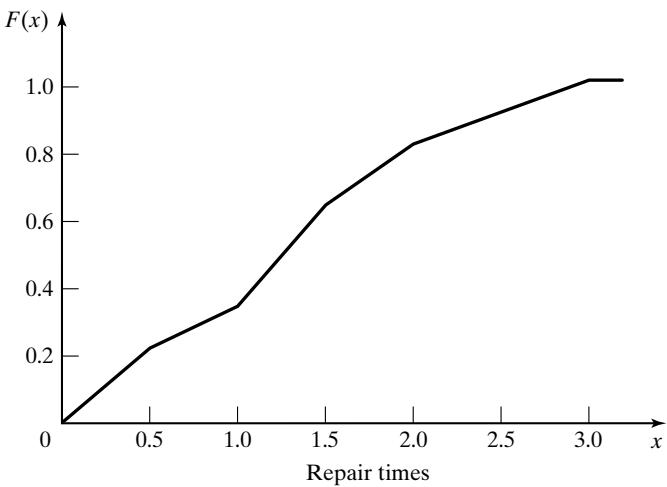 Figure 30 Empirical cdf for repair times.
7 Summary
In many instances, the world the simulation analyst sees is probabilistic rather than deterministic. The purposes of this chapter were to review several important probability distributions, to familiarize the reader with the notation used in the remainder of the text, and to show applications of the probability distributions in a simulation context.
A major task in simulation is the collection and analysis of input data. One of the first steps in this task is hypothesizing a distributional form for the input data. This is accomplished by comparing the shape of the probability density function or mass function to a histogram of the data and by an understanding that certain physical processes give rise to specific distributions. (Computer software is available to assist in this effort.) This chapter was intended to reinforce the properties of various distributions and to give insight into how these distributions arise in practice. In addition, probabilistic models of input data are used in generating random events in a simulation.
Several features that should have made a strong impression on the reader include the differences between discrete, continuous, and empirical distributions; the Poisson process and its properties; and the versatility of the gamma and the Weibull distributions.
REFERENCES
BANKS, J., AND R. G. HEIKES [1984], Handbook of Tables and Graphs for the Industrial Engineer and Manager, Reston Publishing, Reston, VA.
DEVORE, J. L. [1999], Probability and Statisticsfor Engineers and the Sciences, 5th ed., Brooks/Cole, Pacific Grove, CA.
FELLER, W. [1968], An Introduction to Probability Theory and Its Applications, Vol. I, 3d ed., Wiley, NewYork.
GORDON, G. [1975], The Application of GPSS V to Discrete System Simulation, Prentice-Hall, Englewood Cliffs, NJ.
HADLEY, G., AND T. M. WHITIN [1963], Analysis ofInventory Systems, Prentice-Hall, Englewood Cliffs, NJ.
HINES, W. W.,AND D. C. MONTGOMERY [1990], Probability and Statistics in Engineering andManagement Science, 3d ed., Wiley, New York.
LAW, A. M., AND W. D. KELTON [2000], Simulation Modeling & Analysis, 3d ed., McGraw-Hill, New York.
PAPOULIS, A. [1990], Probability and Statistics, Prentice Hall, Englewood Cliffs, NJ.
PARZEN, E. [1999], Stochastic Process, Classics in Applied Mathematics, 24, Society for Industrial & Applied Mathematics, Philadelphia, PA.
PEGDEN, C. D., R. E. SHANNON, AND R. P. SADOWSKI [1995], Introduction to Simulation Using SIMAN, 2d ed., McGraw-Hill, New York
ROSS, S. M. [2002], Introduction to Probability Models, 8th ed., Academic Press, New York.
WALPOLE, R. E., AND R. H. MYERS [2002], Probability and Statisticsfor Engineers and Scientists, 7th ed., Prentice Hall, Upper Saddle River, NJ.
EXERCISES
A production process manufactures alternators for outboard engines used in recreational boating. On the average, 1% of the alternators will not perform up to the required standards when tested at the engine assembly plant. When a large shipment of alternators is received at the plant, 100 are tested, and, if more than two are nonconforming, the shipment is returned to the alternator manufacturer. What is the probability of returning a shipment?
An industrial chemical that will retard the spread of fire in paint has been developed. The loca sales representative has estimated, from past experience, that 48% of the sales calls will resul in an order.
(a) What is the probability that the first order will come on the fourth sales call of the day?
(b) If eight sales calls are made in a day, what is the probability of receiving exactly six orders?
(c) If four sales calls are made before lunch, what is the probability that one or fewer results in an order?
A recent survey indicated that 82% of single women aged 25 years old will be married in their lifetime. Using the binomial distribution, find the probability that two or three women in a sample of twenty will never be married.
The Hawks are currently winning 0.55 of their games. There are 5 games in the next two weeks. What is the probability that they will win more games than they lose?
Joe Coledge is the third-string quarterback for the University of Lower Alatoona. The probability that Joe gets into any game is 0.40.
(a) What is the probability that the first game Joe enters is the fourth game of the season?
(b) What is the probability that Joe plays in no more than two of the first five games?
For the random variables and , which are exponentially distributed with parameter compute 7. Show that the geometric distribution is memoryless.
The number of hurricanes hitting the coast of Florida annually has a Poisson distribution with a mean of 0.8.
(a) What is the probability that more than two hurricanes will hit the Florida coast in a year?
(b) What is the probability that exactly one hurricane will hit the coast of Florida in a year?
- Arrivals at a bank teller’s drive-through window are Poisson-distributed at the rate of 1.2 per minute.
(a) What is the probability of zero arrivals in the next minute?
(b) What is the probability of zero arrivals in the next 2 minutes?
Records indicate that 1.8% of the entering students at a large state university drop out of schoo by midterm. What is the probability that three or fewer students will drop out of a random group of 200 entering students?
Lane Braintwain is quite a popular student. Lane receives, on the average, four phone calls a night (Poisson-distributed). What is the probability that, tomorrow night, the number of calls received will exceed the average by more than one standard deviation?
Lead-time demand for condenser units is Poisson-distributed with a mean of 6 units. Prepare a table for the inventory manager that will indicate the order level to achieve protection of the following levels: 50%, 80%, 90%, 95%, 97%, 97.5%, 99%, 99.5%, and 99.9%.
A random variable X that has pmf given by ) over the range is said to have a discrete uniform distribution.
(a) Find the mean and variance of this distribution. Hint:
(b) If , compute the mean and variance of .
- The lifetime, in years, of a satellite placed in orbit is given by the following pdf:
(a) What is the probability that this satellite is still “alive” after 5 years?
(b) What is the probability that the satellite dies between 3 and 6 years from the time it is placed in orbit?
A mainframe computer crashes in accordance with a Poisson process, with a mean rate of one crash every 36 hours. Determine the probability that the next crash will occur between 24 and 48 hours after the last crash.
(The Poisson distribution can be used to approximate the binomial distribution when n is large and p is small—say, p less than 0.1. In utilizing the Poisson approximation, let In the production of ball bearings, bubbles or depressions occur, rendering the ball bearing unfit for sale. It has been noted that, on the average, one in every 800 of the ball bearings has one or more of these defects. What is the probability that a random sample of 4000 will yield fewer than three ball bearings with bubbles or depressions?
For an exponentially distributed random variable X, find the value of λ that satisfies the following relationship:
Accidents at an industrial site occur one at a time, independently, and completely at random, at a mean rate of one per week. What is the probability that no accidents occur in the next three weeks?
A component has an exponential time-to-failure distribution with mean of 10,000 hours.
(a) The component has already been in operation for its mean life. What is the probability that it will fail by 15,000 hours?
(b) At 15,000 hours, the component is still in operation. What is the probability that it wil operate for another 5000 hours?
- Suppose that a Die-Hardly-Ever battery has an exponential time-to-failure distribution with a mean of 48 months. At 60 months, the battery is still operating.
(a) What is the probability that this battery is going to die in the next 12 months?
(b) What is the probability that the battery dies in an odd year of its life?
(c) If the battery is operating at 60 months, compute the expected additional months of life.
- The time to service customers at a bank teller’s drive-through window is exponentially distributed with a mean of 50 seconds.
(a) What is the probability that the two customers in front of an arriving customer will each take less than 60 seconds to complete their transactions?
(b) What is the probability that the two customers in front will finish their transactions so tha an arriving customer can reach the teller’s window within 2 minutes?
Determine the variance V(X) of the triangular distribution.
The daily use of water, in thousands of liters, at the Hardscrabble Tool and Die Works follows a gamma distribution having shape parameter 2 and scale parameter 1/4. What is the probability that the demand exceeds 4000 liters on any given day?
When Admiral Byrd went to the North Pole, he wore battery-powered thermal underwear. The batteries failed instantaneously rather than gradually. The batteries had a life that was exponentially distributed, with a mean of 12 days. The trip took 30 days. Admiral Byrd packed three batteries. What is the probability that three batteries would be a number sufficient to keep the Admiral warm?
The time intervals between hits on a web page from remote computers are exponentially distributed, with a mean of 15 seconds. Find the probability that the third hit connection occurs after 30 seconds have elapsed.
The rail shuttle cars at theAtlanta airport have a dual electrical braking system.A rail car switches to the standby system automatically if the first system fails. If both systems fail, there will be a crash! Assume that the life of a single electrical braking system is exponentially distributed, with a mean of 4000 operating hours. If the systems are inspected every 5000 operating hours, what is the probability that a rail car will not crash before that time?
Suppose that cars arriving at a toll booth follow a Poisson process with a mean interarrival time of 15 seconds. What is the probability that up to one minute will elapse until three cars have arrived?
Suppose that an average of 30 customers per hour arrive at the Sticky Donut Shop in accordance with a Poisson process. What is the probability that more than 5 minutes will elapse before both of the next two customers walk through the door?
Professor Dipsy Doodle gives six problems on each exam. Each problem requires an average of 30 minutes grading time for the entire class of 15 students. The grading time for each problem is exponentially distributed, and the problems are independent of each other.
(a) What is the probability that the Professor will finish the grading in 2.5 hours or less?
(b) What is the most likely grading time?
(c) What is the expected grading time?
- An aircraft has dual hydraulic systems. The aircraft switches to the standby system automatically if the first system fails. If both systems fail, the plane will crash. Assume that the life of a hydraulic system is exponentially distributed, with a mean of 2000 air hours.
(a) If the hydraulic systems are inspected every 2500 hours, what is the probability that an aircraft will crash before that time?
(b) What danger would there be in moving the inspection point to 3000 hours?
- A random variable X is beta distributed if its pdf is given by
Show that the beta distribution becomes the uniform distribution over the unit interval when 32. Lead time is gamma distributed in 100s of units, with the shape parameter 3 and the scale parameter 1. What is the probability that the lead time exceeds 2 (hundred) units during an upcoming cycle?
Lifetime of an inexpensive video card for a PC, in months, denoted by the random variable X, is gamma distributed with and . What is the probability that the card will last for at least 2 years?
Many states have license plates that conform to the following format:
letter letter letter number number number
The numbers are at random, ranging from 100 to 999.
(a) What is the probability that the next two plates seen (at random) will have numbers of 500 or higher?
(b) What is the probability that the sum of the next two plates seen (at random) will have a tota of 1000 or higher? [Hint: Approximate the discrete uniform distribution with a continuous uniform distribution. The sum of two independent uniform distributions is a triangular distribution.]
Let X be a random variable that is normally distributed, with mean 10 and variance 4. Find the values a and b such that $ P ( a < X < b ) = 0 . 90 {\mathrm{~ a n d ~}} | \mu - a | = | \mu - b |$# Statistical Models in Simulation
Given the following distributions:
Normal (10, 4)
Triangular (4, 10, 16)
Uniform (4, 16)
find the probability that for each of the distributions.
Lead time for an item is approximated by a normal distribution with a mean of 20 days and a variance of 4 days^2. Find values of lead time that will be exceeded only 1%, 5%, and 10% of the time.
IQ scores are normally distributed throughout society, with mean 100 and standard deviation 15.
(a) A person with an IQ of 140 or higher is called a “genius.” What proportion of society is in the genius category?
(b) What proportion of society will miss the genius category by 5 or less points?
(c) Suppose that an IQ of 110 or higher is required to make it through an accredited college or university. What proportion of society could be eliminated from completing a higher education by having a low IQ score?
- Three shafts are made and assembled into a linkage. The length of each shaft, in centimeters, is distributed as follows:
Shaft 1: N(60, 0.09)
Shaft 2: N(40, 0.05)
Shaft 3: N(50, 0.11)
(a) What is the distribution of the length of the linkage?
(b) What is the probability that the linkage will be longer than 150.2 centimeters?
(c) The tolerance limits for the assembly are (149.83, 150.21). What proportion of assemblies are within the tolerance limits? [Hint: If are n independent normal random variables, and if has mean and variance , then the sum
is normal with mean and variance 40. The circumferences of battery posts in a nickel-cadmium battery are Weibull-distributed with centimeters, centimeters, and (a) Find the probability that a battery post chosen at random will have a circumference larger than 3.40 centimeters.
(b) If battery posts are larger than 3.50 centimeters, they will not go through the hole provided; if they are smaller than 3.30 centimeters, the clamp will not tighten sufficiently. Wha proportion of posts will have to be scrapped for one of these reasons?
- The time to failure of a nickel-cadmium battery is Weibull-distributed with parameters ν 0, α 1/2 years, and (a) Find the fraction of batteries that are expected to fail prior to 1.5 years.
(b) What fraction of batteries are expected to last longer than the mean life?
(c) What fraction of batteries are expected to fail between 1.5 and 2.5 years?
Demand for electricity at Gipgip Pig Farm for the merry merry month of May has a triangular distribution, with a 100 kwh and c 1800 kwh. The median kwh is 1425. Compute the modal value of kwh for the month.
The time to failure on an electronic subassembly can be modeled by a Weibull distribution whose location parameter is 0, α 1000 hours, and (a) What is the mean time to failure?
(b) What fraction of these subassemblies will fail by 3000 hours?
The gross weight of three-axle trucks that have been checked at the Hahira Inspection Station on Interstate Highway 85 follows a Weibull distribution with parameters ν 6.8 tons, α 1/2 ton, and β = 1.5. Determine the appropriate weight limit such that 0.01 of the trucks will be cited for traveling overweight.
The current reading on Sag Revas’s gas-mileage indicator is an average of 25.3 miles per gallon. Assume that gas mileage on Sag’s car follows a triangular distribution with a minimum value o zero and a maximum value of 50 miles per gallon. What is the value of the median?
A postal letter carrier has a route consisting of five segments with the time in minutes to complete each segment being normally distributed, with means and variances as shown:
| Tennyson Place | N(38, 16) |
|---|---|
| Windsor Parkway | N(99, 29) |
| Knob Hill Apartments | N(85, 25) |
| Evergreen Drive | N(73, 20) |
| Chastain Shopping Center | N(52, 12) |
In addition to the times just mentioned, the letter carrier must organize the mail at the central office, which activity requires a time that is distributed by N(90, 25). The drive to the starting point of the route requires a time that is distributed N(10, 4). The return from the route requires a time that is distributed N(15, 4). The letter carrier then performs administrative tasks with a time that is distributed N(30, 9).
(a) What is the expected length of the letter carrier’s work day?
(b) Overtime occurs after eight hours of work on a given day. What is the probability that the letter carrier works overtime on any given day?
(c) What is the probability that the letter carrier works overtime on two or more days in a six-day week?
(d) What is the probability that the route will be completed within 24 minutes of eight hours on any given day? [Hint: See Exercise 39.]
The time to failure of a WD-1 computer chip is known to be Weibull-distributed with parameters , and . Find the fraction expected to survive 600 days.
The TV sets on display at Schocker’s Department Store are hooked up such that, when one fails, a model exactly like the one that failed will switch on. Three such units are hooked up in this series arrangement. The lives of these TVs are independent of one another. Each TV has a life which is exponentially distributed, with a mean of 10,000 hours. Find the probability that the combined life of the system is greater than 32,000 hours.
High temperature in Biloxi, Mississippi on July 21, denoted by the random variable X, has the following probability density function, where X is in degrees F.
(a) What is the variance of the temperature V(X)? [Hint: If you worked Exercise 22, this is quite easy.]
(b) What is the median temperature?
(c) What is the modal temperature?
- The time to failure of Eastinghome light bulbs is Weibull-distributed with hours, hours, and (a) What fraction of bulbs are expected to last longer than the mean lifetime?
(b) What is the median lifetime of a light bulb?
Lead-time demand is gamma distributed in 100s of units, with shape parameter 2 and scale parameter 1/4. What is the probability that the lead time exceeds 4 (hundred) units during an upcoming cycle?
Let time correspond to 6 A.M., and suppose that the arrival rate (in arrivals per hour) of customers to a breakfast restaurant that is open from 6 to 9 A.M. is
Assuming an NSPP model is appropriate, do the following: (a) Derive (t). (b) Compute the expected number of arrivals between 6:30 and 8:30 A.M. (c) Compute the probability that there are fewer than 60 arrivals between 6:30 and 8:30 A.M.