8 Random-Variate Generation
This chapter deals with procedures for sampling from a variety ofwidely used continuous and discrete distributions. Previous discussions and examples indicated the usefulness of probability distributions in modeling activities that are generally unpredictable or uncertain. For example, interarrival times and service times at queues and demands for a product are quite often unpredictable in nature, a least to a certain extent. Usually, such variables are modeled as random variables with some specified probability distribution, and standard statistical procedures exist for estimating the parameters of the hypothesized distribution and for testing the validity of the assumed statistical model.
In this chapter, it is assumed that a distribution has been completely specified, and ways are sough to generate samples from this distribution to be used as input to a simulation model. The purpose of the chapter is to explain and illustrate some widely used techniques for generating random variates, not to give a state-of-the-art survey of the most efficient techniques. In practice, most simulation modelers will use either existing routines available in programming libraries or the routines built into a simulation language. However, some programming languages do not have built-in routines for all of the regularly used distributions, and some computer installations do not have random-variategeneration libraries; in such cases the modeler must construct an acceptable routine. Even though the chance of this happening is small, it is nevertheless worthwhile to understand how random-variate generation occurs.
This chapter discusses the inverse-transform technique and, more briefly, the acceptance-rejection technique and special properties. Another technique, the composition method, is discussed by Devroye [1986], Dagpunar [1988], and Law [2007]. All the techniques in this chapter assume that a source of uniform [0,1] random numbers,. is readily available, where each has pdf
and cdf
Throughout this chapter R and . represent random numbers uniformly distributed on [0,1] and generated by random-number generation techniques or taken from a random number table, such as Table A.1 in the Appendix. Many of the algorithms in this chapter have been translated into Visual Basic for Applications and can be found in the spreadsheet RandomNumberTools.xls at www.bcnn.net.
1 Inverse-Transform Technique
The inverse-transform technique can be used to sample from the exponential, uniform, Weibull, and triangular distributions, and from empirical distributions. Additionally, it is the underlying principle for sampling from a wide variety of discrete distributions. The technique will be explained in detai for the exponential distribution and then applied to other distributions. Computationally, it is the most straightforward, but not always the most efficient, technique.
1.1 Exponential Distribution
The exponential distribution has the probability density function (pdf)
and the cumulative distribution function (cdf)
The parameter λ can be interpreted as the mean number of occurrences per time unit. For example, if interarrival times . had an exponential distribution with rate λ, then λ could be interpreted as the mean number of arrivals per time unit, or the arrival rate. Notice that, for any i,
and so is the mean interarrival time. The goal here is to develop a procedure for generating values . that have an exponential distribution.
The inverse-transform technique can be utilized, at least in principle, for any distribution, but it is most useful when the cdf,), is of a form so simple that its inverse,, can be computed easily. (The notation denotes the solution of the equation for x; it does not denote One step-by-step procedure for the inverse-transform technique, illustrated by the exponentia distribution, is shown here:
Step 1. Compute the cdf of the desired random variable For the exponential distribution, the cdf is Step 2. Set on the range of X.
For the exponential distribution, it becomes on the range X is a random variable (with the exponential distribution in this case), so is also a random variable, here called R. As will be shown later, R has a uniform distribution over the interval [0, 1].
Step 3. Solve the equation for X in terms of R.
For the exponential distribution, the solution proceeds as follows:
Equation (1) is called a random-variate generator for the exponential distribution. In general, Equation (1) is written as . Generating a sequence of values is accomplished through Step 4.
Step 4. Generate (as needed) uniform random numbers . and compute the desired random variates by
For the exponential case, by Equation (1), so
for . One simplification that is usually employed in Equation (2) is to replace by to yield
This alternative is justified by the fact that both and are uniformly distributed on [0,1].
Example 1
Table 1 gives a sequence of random numbers from Table A.1 and the computed exponential variates,, given by Equation (2) with the value . Figure 1(a) is a histogram of 200 values, from the uniform distribution, and Figure 1(b) is a histogram of the 200 values,, computed by Equation (2). Compare these empirical histograms with the theoretical density functions in Figure 1(c) and (d). As illustrated here, a histogram is an estimate of the underlying density function.
Table 1 Generation of Exponential Variates with Mean 1, given Random Numbers | i | 1 | 2 | 3 | 4 | 5 |
| 0.1306 | 0.0422 | 0.6597 | 0.7965 | 0.7696 | |
|---|---|---|---|---|---|
| 0.1400 | 0.0431 | 1.078 | 1.592 | 1.468 |
Figure 2 gives a graphical interpretation of the inverse-transform technique. The cdf shown is , an exponential distribution with rate . To generate a value with cdf a random number between 0 and 1 is generated, then a horizontal line is drawn from to the graph of the cdf, then a vertical line is dropped to the x axis to obtain , the desired result. Notice the inverse relation between and , namely
and
In general, the relation is written as
and
Why does the random variable generated by this procedure have the desired distribution? Pick a value and compute the cumulative probability
To see the first equality in Equation (4), refer to Figure 2, where the fixed numbers and are drawn on their respective axes. It can be seen that when and only when ). Since , the second equality in Equation (4) follows immediately from the fact that is uniformly distributed on [0,1]. Equation (4) shows that the cdf of is hence, has the desired distribution.
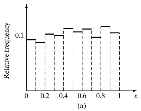
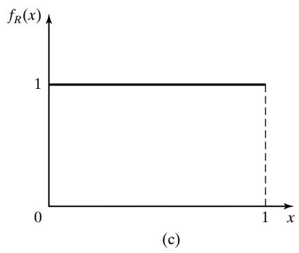
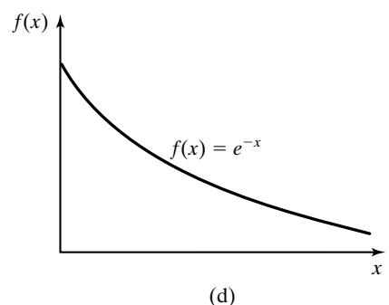
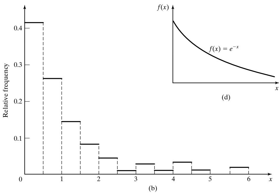 Figure 1 (a) Empirical histogram of 200 uniform random numbers; (b) empirical histogram of 200 exponential variates; (c) theoretical uniform density on [0,1]; (d) theoretical exponentia density with mean 1.
1.2 Uniform Distribution
Consider a random variable X that is uniformly distributed on the interval [a, b]. A reasonable guess for generating X is given by
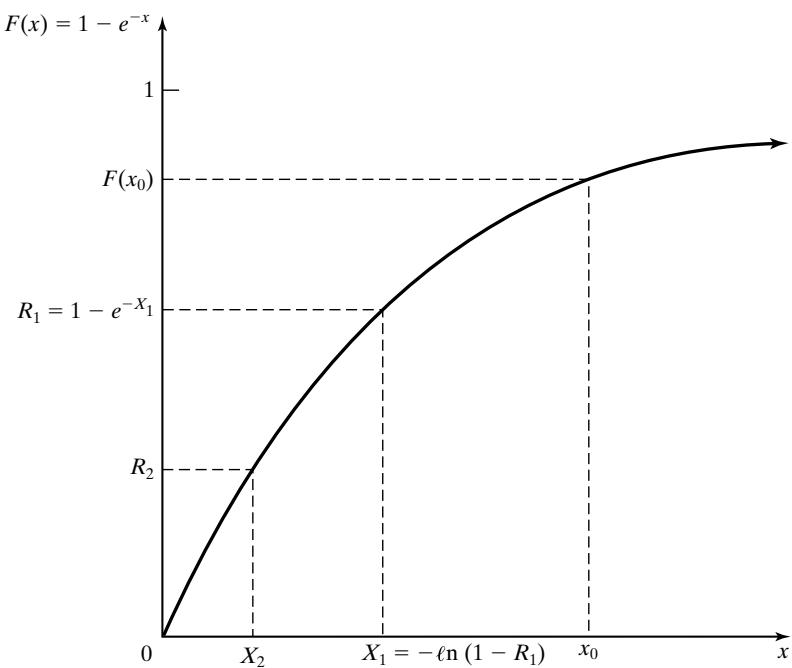 Figure 2 Graphical view of the inverse-transform technique.
(Recall that R is always a random number on [0, 1].) The pdf of X is given by
The derivation of Equation (5) follows Steps 1 through 3 of Section 1.1:
Step 1. The cdf is given by
Step 2. Set Step 3. Solving for X in terms of R yields , which agrees with Equation (5).
1.3 Weibull Distribution
The Weibull distribution was introduced as a model for time to failure for machines or electronic components. When the location parameter ν is set to 0:
where and are the scale and shape parameters of the distribution. To generate a Weibul variate, follow Steps 1 through 3 of Section 1.1:
Step 1. The cdf is given by Step 2. Set Step 3. Solving for X in terms of R yields
The derivation of Equation (6) is left as Exercise 10 for the reader. By comparing Equations (6) and (1), it can be seen that, if X is a Weibull variate, then is an exponential variate with mean Conversely, if Y is an exponential variate with mean , then is a Weibull variate with shape parameter and scale parameter
1.4 Triangular Distribution
Consider a random variable X that has pdf
as shown in Figure 3. This distribution is called a triangular distribution with endpoints and mode at 1. Its cdf is given by
For
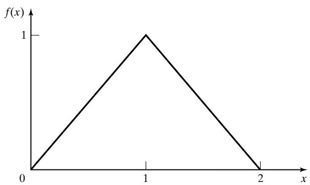 Figure 3 Density function for a particular triangular distribution.
and for
In Equation implies that , in which case . By Equation (8), implies that , in which case . Thus, X is generated by
Exercises 2, 3, and 4 give the student practice in dealing with other triangular distributions. Notice that, if the pdf and cdf of the random variable X come in parts (i.e., require different formulas over different parts of the range of X), then the application of the inverse-transform technique for generating X will result in separate formulas over different parts of the range of R, as in Equation (9).
1.5 Empirical Continuous Distributions
If the modeler has been unable to find a theoretical distribution that provides a good model for the input data, then it may be necessary to use the empirical distribution of the data. One possibility is to simply resample the observed data itself. This is known as using the empirical distribution, and it makes particularly good sense when the input process is known to take on a finite number of values. See Section 1.7 for an example of this type of situation and for a method for generating random inputs.
On the other hand, if the data are drawn from what is believed to be a continuous-valued inpu process, then it makes sense to interpolate between the observed data points to fill in the gaps. This section describes a method for defining and generating data from a continuous empirical distribution.
Five observations of fire-crew response times (in minutes) to incoming alarms have been collected to be used in a simulation investigating possible alternative staffing and crew-scheduling policies. The data are
Before collecting more data, it is desired to develop a preliminary simulation model that uses a response-time distribution based on these five observations. Thus, a method for generating random variates from the response-time distribution is needed. Initially, it will be assumed that response times X have a range , where c is unknown, but will be estimated by , where are the raw data and is the number of observations.
Arrange the data from smallest to largest and let denote these sorted values. The smallest possible value is believed to be 0, so define . Assign the probability to each interval , as shown in Table 2. The resulting empirical cdf, is illustrated in Figure 4. The slope of the ith line segment is given by
The inverse cdf is calculated by
when For example, if a random number is generated, then is seen to lie in the fourth interval (between and ; so, by Equation (10),
The reader is referred to Figure 4 for a graphical view of the generation procedure.
Table 2 Summary of Fire-Crew Response-Time Data
| i | Interval | Probability | Cumulative Probability, i/n | Slope |
|---|---|---|---|---|
| 1 | 0.2 | 0.2 | 4.00 | |
| 2 | 0.2 | 0.4 | 2.20 | |
| 3 | 0.2 | 0.6 | 1.05 | |
| 4 | 0.2 | 0.8 | 1.90 | |
| 5 | 0.2 | 1.0 | 4.65 |
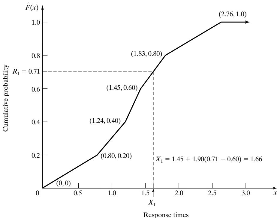 Figure 4 Empirical cdf of fire-crew response times.
In Example 2, each data point was represented in the empirical cdf. If a large sample of data is available (and sample sizes from several hundred to tens of thousands are possible with automated data collection), then it might be more convenient (and computationally efficient) to first summarize the data into a frequency distribution with a much smaller number ofintervals and then fit a continuous empirical cdf to the frequency distribution. Only a slight generalization of Equation (10) is required to accomplish this. Now the slope of the ith line segment is given by:
where is the cumulative probability of the first i intervals of the frequency distribution and is the ith interval. The inverse cdf is calculated as
when Suppose that 100 machine repair times have been collected. The data are summarized in Table 3 in terms of the number of observations in various intervals. For example, there were 31 observations between 0 and 0.5 hour, 10 between 0.5 and 1 hour, and so on. Suppose it is known that all repairs take at least 15 minutes, so that hours always. Then we set , as shown in Table 3 and Figure 5.
Table 3 Summary of Repair-Time Data
| i | Interval (Hours) | Frequency | Relative Frequency | Cumulative Frequency, | Slope |
|---|---|---|---|---|---|
| 1 | 0.25 ≤ x ≤ 0.5 | 31 | 0.31 | 0.31 | 0.81 |
| 2 | 0.5 < x ≤ 1.0 | 10 | 0.10 | 0.41 | 5.0 |
| 3 | 1.0 < x ≤ 1.5 | 25 | 0.25 | 0.66 | 2.0 |
| 4 | 1.5 < x ≤ 2.0 | 34 | 0.34 | 1.00 | 1.47 |
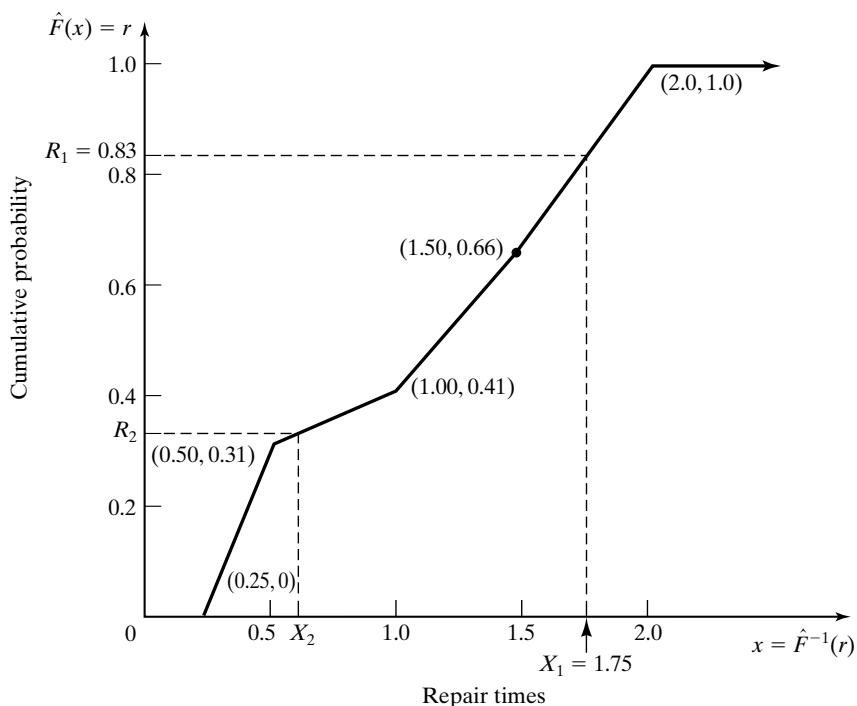 Figure 5 Generating variates from the empirical distribution function for repair-time data For example, suppose the first random number generated is . Then, since is between and
As another illustration, suppose that . Since
The point is also shown in Figure 5.
Now reconsider the data of Table 3. The data are restricted in the range but the underlying distribution might have a wider range. This provides one important reason for attempting to find a theoretical probability distribution (such as the gamma or Weibull) for the data: that these distributions do allow a wider range—namely,. On the other hand, an empirica distribution adheres closely to what is present in the data itself, and the data are often the best source of information available.
When data are summarized in terms of frequency intervals, it is recommended that relatively short intervals be used, for doing so results in a more accurate portrayal of the underlying cdf. For example, for the repair-time data of Table 3, for which there were observations, a much more accurate estimate could have been obtained by using 10 to 20 intervals, certainly not an excessive number, rather than the four fairly wide intervals actually used here for purposes of illustration.
Several comments are in order:
- A computerized version of this procedure will become inefficient as the number of intervals n increases. A systematic computerized version is often called a table-lookup generation scheme, because, given a value of R, the computer program must search an array of values to find the interval i in which R lies, namely the interval i satisfying
The more intervals there are, the longer, on average, the search will take if it is implemented in the crude way described here. The analyst should consider this tradeoff between accuracy of the estimating cdf and computational efficiency when programming the procedure. If a large number of observations are available, the analyst may well decide to group the observations into intervals from 20 to 50, say, and then use the procedure of Example 3—or a more efficient table-lookup procedure could be used, such as the one described in Law [2007].
- In Example 2, it was assumed that response times X satisfied . This assumption led to the inclusion of the points and in Figure 4 and Table 2. If it is known a priori that X falls in some other range—for example, if it is known that response times are always between 15 seconds and 3 minutes, that is,
—then the points and would be used to estimate the empirical cdf of response times. Notice that, because of inclusion of the new point , there are now six intervals instead of five, and each interval is assigned probability . Exercise 12 illustrates the use of these additional assumptions.
1.6 Continuous Distributions without a Closed-Form Inverse
A number of useful continuous distributions do not have a closed form expression for their cdf or its inverse; examples include the normal, gamma, and beta distributions. For this reason, it is often stated that the inverse-transform technique for random-variate generation is not available for these distributions. It can, in effect, become available if we are willing to approximate the inverse cdf, or numerically integrate and search the cdf. Although this approach sounds inaccurate, notice that even a closed-form inverse requires approximation to evaluate it on a computer. For example, generating exponentially distributed random variates via the inverse cdf requires a numerical approximation for the logarithm function. Thus, there is no essential difference between using an approximate inverse cdf and approximately evaluating a closed-form inverse. The problem with using approximate inverse cdfs is that some of them are computationally slow to evaluate.
To illustrate the idea, consider a simple approximation to the inverse cdf of the standard normal distribution, proposed by Schmeiser [1979]:
This approximation gives at least one-decimal-place accuracy for Table 4 compares the approximation with exact values (to four decimal places) obtained by numerical integration for several values of R. Much more accurate approximations exist that are only slightly more complicated. A good source of these approximations for a number of distributions is Bratley, Fox, and Schrage [1996].
Table 4 Comparison of Approximate Inverse with Exact Values (to four decimal places) for the Standard Normal Distribution
| R | Approximate Inverse | Exact Inverse |
|---|---|---|
| 0.01 | -2.3263 | -2.3373 |
| 0.10 | -1.2816 | -1.2813 |
| 0.25 | -0.6745 | -0.6713 |
| 0.50 | 0.0000 | 0.0000 |
| 0.75 | 0.6745 | 0.6713 |
| 0.90 | 1.2816 | 1.2813 |
| 0.99 | 2.3263 | 2.3373 |
1.7 Discrete Distributions
All discrete distributions can be generated via the inverse-transform technique, either numerically through a table-lookup procedure or, in some cases, algebraically, the final generation scheme being in terms of a formula. Other techniques are sometimes used for certain distributions, such as the convolution technique for the binomial distribution. Some of these methods are discussed in later sections. This subsection gives examples covering both empirical distributions and two of the standard discrete distributions, the (discrete) uniform and the geometric. Highly efficient table-lookup procedures for these and other distributions are found in Bratley, Fox, and Schrage [1996] and in Ripley [1987].
Example 4: An Empirical Discrete Distribution
At the end of any day, the number of shipments on the loading dock of the IHW Company is either 0, 1, or 2, with observed relative frequency of occurrence of 0.50, 0.30, and 0.20, respectively. Interna consultants have been asked to develop a model to improve the efficiency of the loading and hauling operations; as part of this model, they will need to be able to generate values X to represent the number of shipments on the loading dock at the end of each day. The consultants decide to model X as a discrete random variable with the distribution given in Table 5 and shown in Figure 6.
Table 5 Distribution of Number of Shipments X
| x | p(x) | F(x) |
|---|---|---|
| 0 | 0.50 | 0.50 |
| 1 | 0.30 | 0.80 |
| 2 | 0.20 | 1.00 |
The probability mass function (pmf), p(x), is given by
and the cdf,, is given by
Recall that the cdf of a discrete random variable always consists of horizontal line segments with jumps of size p(x) at those points, x, that the random variable can assume. For example, in Figure 6, there is a jump of size , of size , and of size at 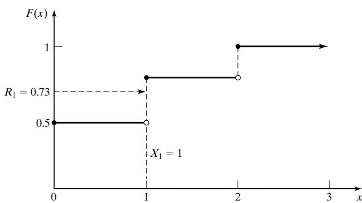 Figure 6 Cdf of number of shipments X.
For generating discrete random variables, the inverse-transform technique becomes a tablelookup procedure, but, unlike in the case of continuous variables, interpolation is not required. To illustrate the procedure, suppose that is generated. Graphically, as illustrated in Figure first locate on the vertical axis, next draw a horizontal line segment until it hits a in the cdf, and then drop a perpendicular to the horizontal axis to get the generated variate. Here is transformed to . This procedure is analogous to the procedure used for empirica continuous distributions in Section 1.5 and illustrated in Figure 4, except that the final step, linear interpolation, is eliminated.
The table-lookup procedure is facilitated by construction of a table such as Table 6. When is generated, first find the interval in which lies. In general, for , if
then set . Here, are the possible values of the random variable; and For this example,, and hence,, and . (Notice that in all cases.)
Table 6 Table for Generating the Discrete Variate X
| Input, | Output, | |
|---|---|---|
| 1 | 0.50 | 0 |
| 2 | 0.80 | 1 |
| 3 | 1.00 | 2 |
Since , set . The generation scheme is summarized as follows:
Example 4 illustrated the table-lookup procedure; the next example illustrates an algebraic approach that can be used for certain distributions.
Example 5: A Discrete Uniform Distribution
Consider the discrete uniform distribution on with pmf and cdf given by
and
Let and . Then, from Inequality (13), it can be seen that, if the generated random number R satisfies
then is generated by setting . Now Inequality (14) can be solved for i:
Let y denote the smallest integer . For example,, and For is a function that rounds up. This notation and Inequality (15) yield a formula for generating X, namely
For example, consider the generating of a random variate X that is uniformly distributed on . The variate X might represent the number of pallets to be loaded onto a truck. Using Table A.1 as a source of random numbers R and using Equation (16) with yields
The procedure discussed here can be modified to generate a discrete uniform random variate with any range consisting of consecutive integers. Exercise 13 asks the student to devise a procedure for one such case.
Example 6: The Geometric Distribution
Consider the geometric distribution with pmf
where . Its cdf is given by
for . Using the inverse-transform technique [i.e., Inequality (13)], recall that a geometric random variable X will assume the value x whenever
where R is a generated random number assumed . Solving Inequality (17) for x proceeds as follows:
But implies that ln , so that
Thus, for that integer value of x satisfying Inequality (18). In brief, and using the round-up function , we have
Since is a fixed parameter, let . Then and, by Equation (19),. By Equation is an exponentially distributed random variable with mean so one way of generating a geometric variate with parameter is to generate (by any method) an exponential variate with parameter , subtract one, and round up.
Occasionally, there is needed a geometric variate X that can assume values q with pm . Such a variate X can be generated, via Equation (19), by
One of the most common cases is
Example 7
Generate three values from a geometric distribution on the range with mean 2. Such a geometric distribution has pmf with mean Thus, X can be generated by Equation (20) with , and . Using Table , and yields
Exercise 15 deals with an application of the geometric distribution.
2 Acceptance-Rejection Technique
Suppose that an analyst needed to devise a method for generating random variates, X, uniformly distributed between 1/4 and 1. One way to proceed would be to follow these steps:
Step 1. Generate a random number R.
Step 2a. If , accept , then go to Step 3.
Step 2b. I , reject R, and return to Step 1.
Step 3. If another uniform random variate on [1/4, 1] is needed, repeat the procedure beginning at Step 1. If not, stop.
Each time Step 1 is executed, a new random number R must be generated. Step 2a is an “acceptance” and Step 2b is a “rejection” in this acceptance-rejection technique. To summarize the technique, random variates R with some distribution (here uniform on [0, 1]) are generated until some condition (here is satisfied. When the condition is finally satisfied, the desired random variate X (here uniform on can be computed . This procedure can be shown to be correct by recognizing that the accepted values of R are conditioned values; that is, R itself does not have the desired distribution, but R conditioned on the event does have the desired distribution. To show this, take ; then
which is the correct probability for a uniform distribution on [1/4, 1]. Equation (21) says that the probability distribution of R, given that R is between 1/4 and 1 (all other values of R are thrown out), is the desired distribution. Therefore, if , set The efficiency of an acceptance-rejection technique depends heavily on being able to minimize the number of rejections. In this example, the probability of a rejection is , so that the number of rejections is a geometrically distributed random variable with probability of “success” being and mean number of rejections . (Example 6 discussed the geometric distribution.) The mean number of random numbers R required to generate one variate X is one more than the number of rejections; hence, it is . In other words, to generate 1000 values of X would require approximately 1333 random numbers R.
In the present situation, an alternative procedure exists for generating a uniform variate on [1/4, 1]—namely, Equation (5), which reduces to . Whether the acceptancerejection technique or an alternative procedure, such as the inverse-transform technique [Equation (5)], is the more efficient depends on several considerations. The computer being used, the skills of the programmer, and the relative inefficiency of generating the additional (rejected) random numbers needed by acceptance-rejection should be compared to the computations required by the alternative procedure. In practice, concern with generation efficiency is left to specialists who conduct extensive tests comparing alternative methods (i.e., until a simulation model begins to require excessive computer runtime due to the generator being used).
For the uniform distribution on [1/4, 1], the inverse-transform technique of Equation (5) is undoubtedly much easier to apply and more efficient than the acceptance-rejection technique. The main purpose of this example was to explain and motivate the basic concept of the acceptancerejection technique. However, for some important distributions, such as the normal, gamma and beta, the inverse cdf does not exist in closed form and therefore the inverse-transform technique is difficult. These more advanced techniques are summarized by Bratley, Fox, and Schrage [1996], and Law [2007].
In the following subsections, the acceptance-rejection technique is illustrated for the generation of random variates for the Poisson, nonstationary Poisson, and gamma distributions.
2.1 Poisson Distribution
A Poisson random variable N with mean has pmf
More important, however, is that N can be interpreted as the number of arrivals from a Poisson arrival process in one unit of time. The interarrival times,. of successive customers are exponentially distributed with rate α (i.e., α is the mean number of arrivals per unit time); in addition, an exponential variate can be generated by Equation (3). Thus, there is a relationship between the (discrete) Poisson distribution and the (continuous) exponential distribution:
if and only if
Equation (22),, says there were exactly n arrivals during one unit of time; but Inequality (23) says that the nth arrival occurred before time 1 while the t arrival occurred after time 1. Clearly, these two statements are equivalent. Proceed now by generating exponential interarriva times until some arrival, say , occurs after time 1; then set For efficient generation purposes, Inequality (23) is usually simplified by first using Equation (3), ln R , to obtain
Next multiply through , which reverses the sign of the inequality, and use the fact that a sum of logarithms is the logarithm of a product, to get
Finally, use the relation for any number x to obtain
which is equivalent to Inequality (23). The procedure for generating a Poisson random variate, N, is given by the following steps:
Step 1. Set
Step 2. Generate a random number , and replace P by Step 3. If , then accept . Otherwise, reject the current n, increase n by one, and return to step 2.
Notice that, upon completion of Step 2, P is equal to the rightmost expression in Inequality (24). The basic idea of a rejection technique is again exhibited; if in Step 3, then n is rejected and the generation process must proceed through at least one more trial.
How many random numbers will be required, on the average, to generate one Poisson variate N? If N n, then n 1 random numbers are required, so the average number is given by
which is quite large if the mean α of the Poisson distribution is large.
Example 8
Generate three Poisson variates with mean . First, compute . Next, get a sequence of random numbers R from Table A.1 and follow the previously described Steps 1 to 3:
Step 1. Step 2. Step 3. Since , accept N 0.
Step 1–3. Step 1. Set Step 2. Step 3. Since , reject n 0 and return to Step 2 with n 1.
Step 2. Step 3. Since , reject n 1 and return to Step 2 with n 2.
Step 2. Step 3. Since , accept N 2.
The calculations required for the generation of these three Poisson random variates are summarized as follows:
| n | P | Accept/Reject | Result | |
|---|---|---|---|---|
| 0 | 0.4357 | 0.4357 | (accept) | N=0 |
| 0 | 0.4146 | 0.4146 | (accept) | N=0 |
| 0 | 0.8353 | 0.8353 | (reject) | |
| 1 | 0.9952 | 0.8313 | (reject) | |
| 2 | 0.8004 | 0.6654 | (accept) | N=2 |
It took five random numbers R to generate three Poisson variates here , and but in the long run, to generate, say, 1000 Poisson variates with mean , it would require approximately or 1200 random numbers.
Example 9
Buses arrive at the bus stop at Peachtree and North Avenue according to a Poisson process with a mean of one bus per 15 minutes. Generate a random variate N which represents the number o arriving buses during a 1-hour time slot. N is Poisson distributed with a mean of four buses per hour. First, compute . Using a sequence of 12 random numbers from Table A.1 yields the following summarized results:
| n | P | Accept/Reject | Result | |
|---|---|---|---|---|
| 0 | 0.4357 | 0.4357 | (reject) | |
| 1 | 0.4146 | 0.1806 | (reject) | |
| 2 | 0.8353 | 0.1508 | (reject) | |
| 3 | 0.9952 | 0.1502 | (reject) | |
| 4 | 0.8004 | 0.1202 | (reject) | |
| 5 | 0.7945 | 0.0955 | (reject) | |
| 6 | 0.1530 | 0.0146 | (accept) | N = 6 |
It is immediately seen that a larger value of α (here usually requires more random numbers; if 1000 Poisson variates were desired, approximately random numbers would be required.
When α is large, say,, the rejection technique outlined here becomes quite expensive, but fortunately an approximate technique based on the normal distribution works quite well. When the mean α is large, then
is approximately normally distributed with mean zero and variance 1; this observation suggests an approximate technique. First, generate a standard normal variate Z, by Equation (28) in Section 3.1, then generate the desired Poisson variate N by
where is the round-up function described in Section 1.7., then set The used in the formula makes the round-up function become a “round to the nearest integer” function. Equation (25) is not an acceptance-rejection technique, but, when used as an alternative to the acceptance-rejection method, it provides a fairly efficient and accurate method for generating Poisson variates with a large mean.
2.2 Nonstationary Poisson Process
Another type of acceptance-rejection method (which is called thinning) can be used to generate interarrival times from a nonstationary Poisson process (NSPP) with arrival rate . An NSPP is an arrival process with an arrival rate that varies with time.
Consider, for instance, the arrival-rate function given in Table 7 that changes every hour. The idea behind thinning is to generate a stationary Poisson arrival process at the fastest rate customer per minute in the example), but “accept” or admit only a portion of the arrivals, thinning out jus enough to get the desired time-varying rate. Next we give the generic algorithm, which generates as the time of the ith arrival. Remember that, in a stationary Poisson arrival process, the times between arrivals are exponentially distributed.
Step 1. Let be the maximum of the arrival rate function and set and Step 2. Generate E from the exponential distribution with rate and let (this is the arrival time of the stationary Poisson process).
Step 3. Generate random number R from the distribution. If then and Step 4. Go to Step 2.
The thinning algorithm can be inefficient if there are large differences between the typical and the maximum arrival rate. However, thinning has the advantage that it works for any integrable arriva rate function, not just a piecewise-constant function, as in this example.
Table 7 Arrival Rate for NSPP Example
| t (min) | Mean Time between Arrivals (min) | Arrival Rate λ(t) (arrivals/min) |
|---|---|---|
| 0 | 15 | 1/15 |
| 60 | 12 | 1/12 |
| 120 | 7 | 1/7 |
| 180 | 5 | 1/5 |
| 240 | 8 | 1/8 |
| 300 | 10 | 1/10 |
| 360 | 15 | 1/15 |
| 420 | 20 | 1/20 |
| 480 | 20 | 1/20 |
Example 10
For the arrival-rate function in Table 7, generate the first two arrival times.
Step 1. Step 2. For random number R 0.2130, E 5 ln(0.213) 13.13 and t 0 13.13 13.13.
Step 3. Generate . Since , do not generate the arrival.
Step 4. Go to Step 2.
Step 2. For random number Step 3. Generate t 16.09 and i i 12.
Step 4. Go to Step 2.
Step 2. For random number 62.14.
Step 3. Generate . Since , set t 62.14 and i i 13.
Step 4. Go to Step 2.
2.3 Gamma Distribution
Several acceptance-rejection techniques for generating gamma random variates have been developed. (See Bratley, Fox, and Schrage [1996] and Law [2007].) One ofthe more efficient is by Cheng [1977]; the mean number of trials is between 1.13 and 1.47 for any value of the shape parameter If the shape parameter is an integer, say,, one possibility is to use the convolution technique in Example 12, because the Erlang distribution is a special case of the more genera gamma distribution. On the other hand, the acceptance-rejection technique described here would be a highly efficient method for the Erlang distribution, especially if were large. The routine generates gamma random variates with scale parameter θ and shape parameter —that is, with mean and variance The steps are as follows
Step 1. Compute Step 2. Generate and . Set Step 3. Compute Step 4a. If ), reject X and return to Step 2.
Step 4b. If , use X as the desired variate.
The generated variates from Step 4b will have mean and variance both equal to . If it is desired to have mean and variance , then include Step 5.
(Step 5. Replace X by )
The basic idea of all acceptance-rejection methods is again illustrated here, but the proof of this example is beyond the scope of this text. In Step 3, is not gamma distributed, but rejection of certain values of X in Step 4a guarantees that the accepted values in Step 4b do have the gamma distribution.
Example 11
Downtimes for a high-production candy-making machine have been found to be gamma distributed with mean 2.2 minutes and variance 2.10 minutes^2. Thus, and , which together imply that β 2.30 and θ 0.4545.
Step 1. a 0.53, b 0.91.
Step 2. Generate R 0.832, R 0.021. Set V 0.832/(10.832) 4.952.
Step 3. Compute X 2.3(4.952)0.53 5.37.
Step 4. X 5.37 > 0.91 [2.3(0.53) 1] ln(4.952) ln[(0.832)^20.021] 8.68, so reject X and return to Step 2.
Step 2. Generate Step 3. Compute X 2.3(0.767)0.53 2.00.
Step 4. Since X 2.000.91 [2.3(0.53) 1] ln(0.767) ln[(0.434)^20.716] 2.32, accept X.
Step 5. Divide X by βθ 1.045 to get X 1.91.
This example took two trials (i.e., one rejection) to generate an acceptable gamma-distributed random variate, but, on the average, to generate, say, 1000 gamma variates, the method will require between 1130 and 1470 trials, or equivalently, between 2260 and 2940 random numbers. The method is somewhat cumbersome for hand calculations, but is easy to program on the computer and is one of the most efficient gamma generators known.
3 Special Properties
“Special properties” are just as the name implies: They are variate-generation techniques that are based on features of a particular family of probability distributions, rather than being general-purpose techniques like the inverse-transform or acceptance-rejection techniques.
3.1 Direct Transformation for the Normal and Lognormal Distributions
Many methods have been developed for generating normally distributed random variates. The inversetransform technique cannot easily be applied, however, because the inverse cdf cannot be written in closed form. The standard normal cdf is given by
This section describes an intuitively appealing direct transformation that produces an independen pair of standard normal variates with mean zero and variance 1. The method is due to Box and Muller [1958]. Although not as efficient as many more modern techniques, it is easy to program in a scientific language, such as FORTRAN, C, C , Visual Basic, or Java. We then show how to transform a standard normal variate into a normal variate with mean and variance . Once we have a method (this or any other) for generating from an distribution, then we can generate a lognorma random variate with parameters and by using the direct transformation . (Recall that and are not the mean and variance of the lognormal.)
Consider two standard normal random variables, and , plotted as a point in the plane as shown in Figure 7 and represented in polar coordinates as
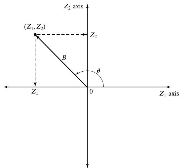 Figure 7 Polar representation of a pair of standard normal variables.
It is known that has the chi-square distribution with 2 degrees of freedom, which is equivalent to an exponential distribution with mean 2. Thus, the radius B can be generated by use of Equation (3):
By the symmetry of the normal distribution, it seems reasonable to suppose, and indeed it is the case, that the angle is uniformly distributed between 0 and 2π radians. In addition, the radius B and the angle are mutually independent. Combining Equations (26) and (27) gives a direct method for generating two independent standard normal variates. and , from two independent random numbers, and
To illustrate the generation scheme, consider Equation (28) with and Two standard normal random variates are generated as follows:
To obtain normal variates X_i with mean and variance , we then apply the transformation
to the standard normal variates. For example, to transform the two standard normal variates into normal variates with mean and variance , we compute
Recall that to obtain a lognormal variate Y from a normal variate X we set . Also recal that the mean and variance of the lognormal Y is not the same as the normal X.
3.2 Convolution Method
The probability distribution of a sum of two or more independent random variables is called a convolution of the distributions of the original variables. The convolution method thus refers to adding together two or more random variables to obtain a new random variable with the desired distribution. This technique can be applied to obtain Erlang variates and binomial variates. What is important is not the cdf of the desired random variable, but rather its relation to other variates more easily generated.
Example 12: Erlang Distribution
An Erlang random variable X with parameters can be shown to be the sum of k independen exponential random variables,, each having mean —that is,
The convolution approach is to generate , then sum them to get X. In the case of the Erlang, each X can be generated by Equation (3) with . Therefore, an Erlang variate can be generated by
It is more efficient computationally to multiply all the random numbers first and then to compute only one logarithm.
Example 13
Trucks arrive at a large warehouse in a completely random fashion that is modeled as a Poisson process with arrival rate trucks per hour. The guard at the entrance sends trucks alternately to the north and south docks. An analyst has developed a model to study the loading/unloading process at the south docks and needs a model of the arrival process at the south docks alone. An interarrival time X between successive truck arrivals at the south docks is equal to the sum of two interarrival times at the entrance and thus it is the sum of two exponential random variables, each having mean 0.1 hour, or 6 minutes. Thus, X has the Erlang distribution with and mean hour. To generate the variate first obtain random numbers from Table A.1, say and . Then, by Equation (30),
In general, Equation (30) implies that k uniform random numbers are needed for each Erlang variate generated. If k is large, it is more efficient to generate Erlang variates by other techniques, such as one of the many acceptance-rejection techniques for the gamma distribution given in Section 2.3, or by Bratley, Fox and Schrage [1996] and Law [2007].
3.3 More Special Properties
There are many relationships among probability distributions that can be exploited for random-variate generation. The convolution method in the Section 3.2 is one example. Another particularly usefu example is the relationship between the beta distribution and the gamma distribution.
Suppose that has a gamma distribution with shape parameter and scale parameter , while has a gamma distribution with shape parameter and scale parameter and that these two random variables are independent. Then
has a beta distribution with parameters and on the interval [0, 1]. If, instead, we want to be defined on the interval , then set
Thus, using the acceptance-rejection technique for gamma variates defined in the previous section, we can generate beta variates, with two gamma variates required for each beta
Although this method of beta generation is convenient, there are faster methods based on acceptance-rejection ideas. See, for instance, Devroye [1986] or Dagpunar [1988].
4 Summary
The basic principles ofrandom-variate generation via the inverse-transform technique, the acceptancerejection technique, and special properties have been introduced and illustrated by examples. Methods for generating many of the important continuous and discrete distributions, plus all empirical distributions, have been given. See Schmeiser [1980] for an excellent survey; for advanced treatments the reader is referred to Devroye [1986] or Dagpunar [1988].
REFERENCES
BRATLEY, P., B. L. FOX, AND L. E. SCHRAGE [1996], A Guide to Simulation, 2d ed., Springer-Verlag, New York.
BOX, G. E. P., AND M. F. MULLER [1958], “A Note on the Generation of Random Normal Deviates,” Annals ofMathematical Statistics, Vol. 29, pp. 610–611.
CHENG, R. C. H. [1977], “The Generation of Gamma Variables with Nonintegral Shape Parameter,” Applied Statistics, Vol. 26, No. 1, pp. 71–75.
DAGPUNAR, J. [1988], Principles ofRandom Variate Generation, Clarendon Press, Oxford.
DEVROYE, L. [1986], Non-Uniform Random Variate Generation, Springer-Verlag, New York.
LAW, A. M. [2007], Simulation Modeling and Analysis, 4th ed., McGraw-Hill, New York.
RIPLEY, B. D. [1987], Stochastic Simulation, Wiley, New York.
SCHMEISER, B. W. [1979], “Approximations to the Inverse Cumulative Normal Function for Use on Hand Calculators,” Applied Statistics, Vol. 28, pp. 175–176.
SCHMEISER, B. W. [1980], “Random Variate Generation: A Survey,” in Simulation with Discrete Models: A State ofthe Art View, T. I. Oren, C. M. Shub, and P. F. Roth, eds., IEEE, NY, pp. 79–104.¨
EXERCISES
Many of the exercises in this section ask the reader to develop a generation scheme for a given distribution and generate values. The results should be implemented in a programming language or spreadsheet so that large numbers of variates can be generated.
- Develop a random-variate generator for a random variable X with the pdf
- Develop a generation scheme for the triangular distribution with pdf
Generate 1000 values of the random variate, compute the sample mean, and compare it to the true mean of the distribution.
Develop a generator for a triangular distribution with range (1, 10) and mode at Generate 1000 values of the random variate, compute the sample mean, and compare it to the true mean of the distribution.
Develop a generator for a triangular distribution with range (1, 10) and a mean of 4. Generate 1000 values of the random variate, compute the sample mean, and compare it to the true mean of the distribution.
Given the following cdf for a continuous variable with range from 3 to 4, develop a generator for the variable, generate 1000 values, and plot a histogram.
Given the cdf , develop a generator for this distribution. Generate 1000 values of the random variate, compute the sample mean, and compare it to the true mean of the distribution.
Given the pdf , develop a generator for this distribution. Generate 1000 values of the random variate, compute the sample mean, and compare it to the true mean of the distribution.
Develop a generator for a random variable whose pdf is
Generate 1000 values and plot a histogram.
- The cdf of a discrete random variable X is given by
When , generate three values of X, using , and 10. Times to failure for an automated production process have been found to be randomly distributed with a Weibull distribution with parameters and . Derive Equation (6), and then use it to generate five values from this Weibull distribution, using five random numbers taken from Table A.1.
- Data have been collected on service times at a drive-in bank window at the Shady Lane National Bank. This data are summarized into intervals as follows:
| Interval (Seconds) | Frequency |
|---|---|
| 15–30 | 10 |
| 30–45 | 20 |
| 45–60 | 25 |
| 60–90 | 35 |
| 90–120 | 30 |
| 120–180 | 20 |
| 180–300 | 10 |
Set up a table like Table 3 for generating service times by the table-lookup method, and generate five values of service time, using four-digit random numbers from Table A.1.
In Example 2, assume that fire-crew response times satisfy . Modify Table 2 to accommodate this assumption. Then generate five values of response time, using four-digi uniform random numbers from Table A.1.
For a preliminary version of a simulation model, the number of pallets X to be loaded onto a truck at a loading dock was assumed to be uniformly distributed between 8 and 24. Devise a method for generating X, assuming that the loads on successive trucks are independent. Use the technique of Example 5 for discrete uniform distributions. Finally, generate loads for 10 successive trucks by using four-digit random numbers from Table A.1.
Develop a method for generating values from a negative binomial distribution with parameters p and k. Generate 3 values when and . [Hint: Think about the definition of the negative binomial as the number of Bernoulli trials until the kth success.]
The weekly demand X for a slow-moving item has been found to be approximated well by a geometric distribution on the range with mean weekly demand of 2.5 items. Generate 10 values of X demand per week, using random numbers from Table A.1. [Hint: For a geometric distribution on the range with parameter p, the mean is 16. In Exercise 15, suppose that the demand has been found to have a Poisson distribution with mean 2.5 items per week. Generate 10 values of X demand per week, using random numbers from Table A.1. Discuss the differences between the geometric and the Poisson distributions.
Lead times have been found to be exponentially distributed with mean 3.7 days. Generate five random lead times from this distribution.
Regular maintenance of a production routine has been found to vary and has been modeled as a normally distributed random variable with mean 33 minutes and variance 4 minutes^2. Generate five random maintenance times from the given distribution.
A machine is taken out of production either if it fails or after 5 hours, whichever comes first. By running similar machines until failure, it has been found that time to failure X has the Weibull distribution with , and ν 0. Thus, the time until the machine is taken out of production can be represented as . Develop a step-by-step procedure for generating Y.
The time until a component is taken out of service is uniformly distributed on from 0 to 8 hours. Two such independent components are put in series, and the whole system goes down when one of the components goes down. If represents the component runtimes, then represents the system lifetime. Devise two distinct ways to generate Y. [Hint: One way is relatively straightforward. For a second method, first compute the cdf of Y :, for . Use the equivalence and and the independence of , and . After finding ), proceed with the inversetransform technique.]
In Exercise 20, component lifetimes are exponentially distributed, one with mean 2 hours and the other with mean 6 hours. Rework Exercise 20 under this new assumption. Discuss the relative efficiency of the two generation schemes devised.
Develop a technique for generating a binomial random variable X via the convolution technique. [Hint: X can be represented as the number of successes in n independent Bernoulli trials, each success having probabilityp. Thus,, where and 23. Develop an acceptance-rejection technique for generating a geometric random variable X with parameter p on the range . [Hint: X can be thought of as the number of failures before the first success occurs in a sequence of independent Bernoulli trials.]
Write a computer routine to generate standard normal variates by the exact method discussed in this chapter. Use it to generate 10,000 values. Compare the true probability,, that a value lies in to the actual observed relative frequency that values were , and 4.
Write a computer routine to generate gamma variates with shape parameter and scale parameter θ. Generate 1000 values with and and compare the true mean,, to the sample mean.
Write a computer routine to generate 2000 values from one of the variates in Exercises 1 to 23. Make a histogram of the 2000 values and compare it to the theoretical density function (or probability mass function for discrete random variables).
Many spreadsheet, symbolic-calculation, and statistical-analysis programs have built-in routines for generating random variates from standard distributions. Try to find out what variate-generation methods are used in one of these packages by looking at the documentation. Should you trust a variate generator if the method is not documented?
Suppose that, somehow, we have available a source of exponentially distributed random variates with mean 1. Write an algorithm to generate random variates with a triangular distribution by transforming the exponentially distributed random variates. [Hint: First, transform to obtain uniformly distributed random variates.]
Let time t 0 correspond to 6 A.M., and suppose that the arrival rate (in arrivals per hour) of customers to a breakfast restaurant that is open 6–9 A.M. is
Derive a thinning algorithm for generating arrivals from this NSPP and generate the first 100 arrival times.
Generate 10 values from a beta distribution on the interval [0, 1] with parameters and . Next transform them to be on the interval [ 10, 20]
Suppose that a discrete distribution can take values . These values are equally likely, but are not . Come up with a generation scheme that exploits the idea in Example 5. [Hint: Consider storing the values in an array, then generating a random array index.]
Suppose that the arrival rate of hits to a web site is hits per hour. Derive a thinning algorithm for generating arrivals from this NSPP.
List of Materials Available on www.bcnn.net
RandomNumberTools.xls