10 Verification and Validation of Simulation Models
One ofthe most important and difficult tasks facing a model developer is the verification and validation of the simulation model. The engineers and analysts who use the model outputs to aid in making design recommendations and the managers who make decisions based on these recommendations— justifiably look upon a model with some degree of skepticism about its validity. It is the job o the model developer to work closely with the end users throughout the period of development and validation to reduce this skepticism and to increase the model’s credibility.
The goal of the validation process is twofold: (a) to produce a model that represents true system behavior closely enough for the model to be used as a substitute for the actual system for the purpose of experimenting with the system, analyzing system behavior, and predicting system performance; and (b) to increase the credibility of the model to an acceptable level, so that the model will be used by managers and other decision makers.
Validation should not be seen as an isolated set of procedures that follows model development, but rather as an integral part of model development. Conceptually, however, the verification and validation process consists of the following components:
Verification is concerned with building the model correctly. It proceeds by the comparison of the conceptual model to the computer representation that implements that conception. It asks the questions: Is the model implemented correctly in the simulation software? Are the input parameters and logical structure of the model represented correctly?
Validation is concerned with building the correct model. It attempts to confirm that a mode is an accurate representation of the real system. Validation is usually achieved through the calibration ofthe model, an iterative process ofcomparing the model to actual system behavior and using the discrepancies between the two, and the insights gained, to improve the model. This process is repeated until model accuracy is judged to be acceptable.
This chapter describes methods that have been recommended and used in the verification and validation process. Most of the methods are informal subjective comparisons; a few are forma statistical procedures. The use of the latter procedures involves issues related to output analysis. Output analysis refers to analysis of the data produced by a simulation and to drawing inferences from these data about the behavior of the real system. To summarize their relationship, validation is the process by which model users gain confidence that output analysis is making valid inferences about the real system under study.
Many articles and chapters in texts have been written on verification and validation. For discussion of the main issues, the reader is referred to Balci [1994, 1998, 2003], Carson [1986, 2002], Gass [1983], Kleijnen [1995], Law and Kelton [2000], Naylor and Finger [1967], Oren [1981], Sargen [2003], Shannon [1975], and van Horn [1969, 1971]. For statistical techniques relevant to various aspects of validation, the reader can obtain the foregoing references plus those by Balci and Sargen [1982a,b; 1984a], Kleijnen [1987], and Schruben [1980]. For case studies in which validation is emphasized, the reader is referred to Carson et al. [1981a,b], Gafarian and Walsh [1970], Kleijnen [1993], and Shechter and Lucas [1980]. Bibliographies on validation have been published by Balc and Sargent [1984b] and by Youngblood [1993].
1 Model Building, Verification, and Validation
The first step in model building consists of observing the real system and the interactions among its various components and of collecting data on their behavior. But observation alone seldom yields sufficient understanding of system behavior. People familiar with the system, or any subsystem, should be questioned, to take advantage of their special knowledge. Operators, technicians, repair and maintenance personnel, engineers, supervisors, and managers understand certain aspects of the system that might be unfamiliar to others. As model development proceeds, new questions may arise, and the model developers will return to this step to learn more about system structure and behavior.
The second step in model building is the construction of a conceptual model—a collection of assumptions about the components and the structure of the system, plus hypotheses about the values of model input parameters. As is illustrated by Figure 1, conceptual validation is the comparison o the real system to the conceptual model.
The third step is the implementation of an operational model, usually by using simulation software, and incorporating the assumptions ofthe conceptual model into the worldview and concepts of the simulation software.
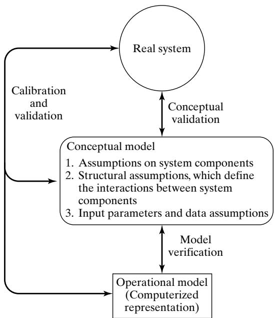 Figure 1 Model building, verification, and validation.
In actuality, model building is not a linear process with three steps. Instead, the model builder will return to each of these steps many times while building, verifying, and validating the model. Figure 1 depicts the ongoing model building process, in which the need for verification and validation causes continual comparison of the real system to both the conceptual model and the operationa model, and induces repeated modification of the model to improve its accuracy.
2 Verification of Simulation Models
The purpose of model verification is to assure that the conceptual model is reflected accurately in the operational model. The conceptual model quite often involves some degree of abstraction about system operations or some amount of simplification of actual operations. Verification asks the following question: Is the conceptual model (assumptions about system components and system structure, parameter values, abstractions, and simplifications) accurately represented by the operationa model?
Many common-sense suggestions can be used in the verification process:
Have the operational model checked by someone other than its developer, preferably an expert in the simulation software being used.
Make a flow diagram that includes each logically possible action a system can take when an event occurs, and follow the model logic for each action for each event type.
Closely examine the model output for reasonableness under a variety of settings of the input parameters. Have the implemented model display a wide variety of output statistics, and examine all of them closely.
Have the operational model print the input parameters at the end of the simulation, to be sure that these parameter values have not been changed inadvertently.
Make the operational model as self-documenting as possible. Give a precise definition of every variable used and a general description of the purpose of each submodel, procedure (or major section of code), component, or other model subdivision.
If the operational model is animated, verify that what is seen in the animation imitates the actual system. Examples of errors that can be observed through animation are automated guided vehicles (AGVs) that pass through one another on a unidirectional path or at an intersection and entities that disappear (unintentionally) during a simulation.
The Interactive Run Controller (IRC) or debugger is an essential component of successfu simulation model building. Even the best of simulation analysts makes mistakes or commits logical errors when building a model. The IRC assists in finding and correcting those errors in the following ways:
(a) The simulation can be monitored as it progresses. This can be accomplished by advancing the simulation until a desired time has elapsed, then displaying model information at that time. Another possibility is to advance the simulation until a particular condition is in effect, and then display information.
(b) Attention can be focused on a particular entity, line of code, or procedure. For instance, every time that an entity enters a specified procedure, the simulation will pause so that information can be gathered. As another example, every time that a specified entity becomes active, the simulation will pause.
(c) Values of selected model components can be observed. When the simulation has paused, the current value or status of variables, attributes, queues, resources, counters, and so on can be observed.
(d) The simulation can be temporarily suspended, or paused, not only to view information, but also to reassign values or redirect entities.
- Graphical interfaces are recommended for accomplishing verification and validation [Bortscheller and Saulnier, 1992]. The graphical representation of the model is essentially a form of self-documentation. It simplifies the task of understanding the model.
These suggestions are basically the same ones any software engineer would follow.
Among these common-sense suggestions, one that is very easily implemented, but quite often overlooked, especially by students who are learning simulation, is a close and thorough examination of model output for reasonableness (suggestion 3). For example, consider a model of a complex network of queues consisting of many service centers in series and parallel configurations. Suppose that the modeler is interested mainly in the response time, defined as the time required for a customer to pass through a designated part of the network. During the verification (and calibration) phase of model development, it is recommended that the program collect and print out many statistics in addition to response times, such as utilizations of servers and time-average number of customers in various subsystems. Examination of the utilization of a server, for example, might reveal that it is unreasonably low (or high), a possible error that could be caused by wrong specification of mean service time, or by a mistake in model logic that sends too few (or too many) customers to this particular server, or by any number of other possible parameter misspecifications or errors in logic.
In a simulation language that automatically collects many standard statistics (average queue lengths, average waiting times, etc.), it takes little or no extra programming effort to display almost all statistics of interest. The effort required can be considerably greater in a general-purpose language such as C, C++, or Java, which do not have statistics-gathering capabilities to aid the programmer.
Two sets ofstatistics that can give a quick indication ofmodel reasonableness are current contents and total count. These statistics apply to any system having items of some kind flowing through it, whether these items be called customers, transactions, inventory, or vehicles. Current contents refers to the number of items in each component of the system at a given time. Total count refers to the tota number of items that have entered each component of the system by a given time. In some simulation software, these statistics are kept automatically and can be displayed at any point in simulation time. In other simulation software, simple counters might have to be added to the operational mode and displayed at appropriate times. If the current contents in some portion of the system are high, this condition indicates that a large number of entities are delayed. If the output is displayed for successively longer simulation run times and the current contents tend to grow in a more or less linear fashion, it is highly likely that a queue is unstable and that the server(s) will fall further behind as time continues. This indicates possibly that the number of servers is too small or that a service time is misspecified On the other hand if the total count for some subsystem is zero this indicates that no items entered that subsystem—again, a highly suspect occurrence. Another possibility is tha the current count and total count are equal to one. This could indicate that an entity has captured a resource, but never freed that resource. Careful evaluation of these statistics for various run lengths can aid in the detection of mistakes in model logic and data misspecifications. Checking for outpu reasonableness will usually fail to detect the more subtle errors, but it is one of the quickest ways to discover gross errors. To aid in error detection, it is best for the model developer to forecast a reasonable range for the value of selected output statistics before making a run of the model. Such a forecast reduces the possibility of rationalizing a discrepancy and failing to investigate the cause o unusual output.
For certain models, it is possible to consider more than whether a particular statistic is reasonable. It is possible to compute certain long-run measures of performance. For example, the analys can compute the long-run server utilization for a large number of queueing systems without any special assumptions regarding interarrival or service-time distributions. Typically, the only information needed is the network configuration, plus arrival and service rates. Any measure of performance that can be computed analytically and then compared to its simulated counterpart provides another valuable tool for verification. Presumably, the objective of the simulation is to estimate some measure of performance, such as mean response time, that cannot be computed analytically; but, all the measures of performance in a queueing system are interrelated. Thus, if a simulation mode is predicting one measure (such as utilization) correctly, then confidence in the model’s predictive ability for other related measures (such as response time) is increased (even though the exact rela tion between the two measures is, of course, unknown in general and varies from model to model). Conversely, if a model incorrectly predicts utilization, its prediction of other quantities, such as mean response time, is highly suspect.
Another important way to aid the verification process is the oft-neglected documentation phase. If a model builder writes brief comments in the operational model, plus definitions of all variables and parameters, plus descriptions of each major section of the operational model, it becomes much simpler for someone else, or the model builder at a later date, to verify the model logic. Documentation is also important as a means of clarifying the logic of a model and verifying its completeness.
A more sophisticated technique is the use of a trace. In general, a trace provides detailed, timestamped simulation output representing the values for a selected set of system states, entity attributes, and model variables whenever an event occurs. That is, at the time an event occurs, the model would write detailed status information to a file for later examination by the model developer to assist in model verification and the detection of modeling errors
Example 1
When verifying the operational model (in a general-purpose language such as C, C++ or Java, or most simulation languages) of the single-server queue model of Example 5 from the “Simulation Examples in a Spreadsheet” chapter, an analyst made a run over 16 units of time and observed that the time-average length of the waiting line was customer, which is certainly reasonable for a short run of only 16 time units. Nevertheless, the analyst decided that a more detailed verification would be of value.
The trace in Figure 2 gives the hypothetical trace output from simulation time CLOCK 0 to CLOCK 16 for the simple single-server queue of Example 5 from the “Simulation Examples in a Spreadsheet” chapter. This example illustrates how an error can be found with a trace, when no error was apparent from the examination of the summary output statistics (such as . Note that, at simulation time CLOCK 3, the number of customers in the system is , but the server is idle (STATUS 0). The source of this error could be incorrect logic, or simply not setting the attribute STATUS to the value 1 (when coding in a general-purpose language or most simulation languages).
In any case, the error must be found and corrected. Note that the less sophisticated practice of examining the summary measures, or output, did not detect the error. By using equation , the reader can verify that was computed correctly from the data is the time-average value of NCUST minus STATUS):
as previously mentioned. Thus, the output measure had a reasonable value and was computed correctly from the data, but its value was indeed wrong because the attribute STATUS was not assuming correct values. As is seen from Figure 2, a trace yields information on the actual history of the model that is more detailed and informative than the summary measures alone.
Most simulation software has a built-in capability to conduct a trace without the programmer having to do any extensive programming. In addition, a ‘print’ or ‘write’ statement can be used to implement a tracing capability in a general-purpose language.
As can be easily imagined, a trace over a large span of simulation time can quickly produce an extremely large amount of output, which would be extremely cumbersome to check in detail for correctness. The purpose of the trace is to verify the correctness of the computer program by making detailed paper-and-pencil calculations. To make this practical, a simulation with a trace is usually
Figure 2 Simulation Trace.
restricted to a very short period of time. It is desirable, of course, to ensure that each type of event (such as Arrival) occurs at least once, so that its consequences and effect on the model can be checked for accuracy. If an event is especially rare in occurrence, it may be necessary to use artificial data to force it to occur during a simulation of short duration. This is legitimate, as the purpose is to verify that the effect on the system of the rare event is as intended.
Some software allows a selective trace. For example, a trace could be set for specific locations in the model or could be triggered to begin at a specified simulation time. Whenever an entity goes through the designated locations, the simulation software writes a time-stamped message to a trace file. Some simulation software allows for tracing a selected entity; any time the designated entity becomes active, the trace is activated and time-stamped messages are written. This trace is very useful in following one entity through the entire model. Another example of a selective trace is to set it for the occurrence of a particular condition. For example, whenever the queue before a certain resource reaches five or more, turn on the trace. This allows running the simulation until something unusual occurs, then examining the behavior from that point forward in time. Different simulation software packages support tracing to various extents. In practice, it is often implemented by the model developer by adding printed messages at appropriate points into a model.
Of the three classes of techniques—the common-sense techniques, thorough documentation, and traces—it is recommended that the first two always be carried out. Close examination of mode output for reasonableness is especially valuable and informative. A generalized trace may provide voluminous data, far more than can be used or examined carefully. A selective trace can provide useful information on key model components and keep the amount of data to a manageable level.
3 Calibration and Validation of Models
Calibration and validation, although conceptually distinct, usually are conducted simultaneously by the modeler. Validation is the overall process of comparing the model and its behavior to the rea system and its behavior. Calibration is the iterativeprocess of comparing the model to the real system, making adjustments (or even major changes) to the model, comparing the revised model to reality, making additional adjustments, comparing again, and so on. Figure 3 shows the relationship of mode calibration to the overall validation process. The comparison of the model to reality is carried out by a variety of tests—some subjective, others objective. Subjective tests usually involve people, who are knowledgeable about one or more aspects of the system, making judgments about the model and its output. Objective tests always require data on the system’s behavior, plus the corresponding data produced by the model. Then one or more statistical tests are performed to compare some aspect of the system data set with the same aspect of the model data set. This iterative process of comparing model with system and then revising both the conceptual and operational models to accommodate any perceived model deficiencies is continued until the model is judged to be sufficiently accurate.
A possible criticism of the calibration phase, were it to stop at this point, is that the model has been validated only for the one data set used—that is, the model has been “fitted” to one data set. One way to alleviate this criticism is to collect a new set of system data (or to reserve a portion of the original system data) to be used at this final stage of validation. That is, after the model has been calibrated by using the original system data set, a “final” validation is conducted, using the second system data set. If unacceptable discrepancies between the model and the real system are discovered in the “final” validation effort, the modeler must return to the calibration phase and modify the mode until it becomes acceptable.
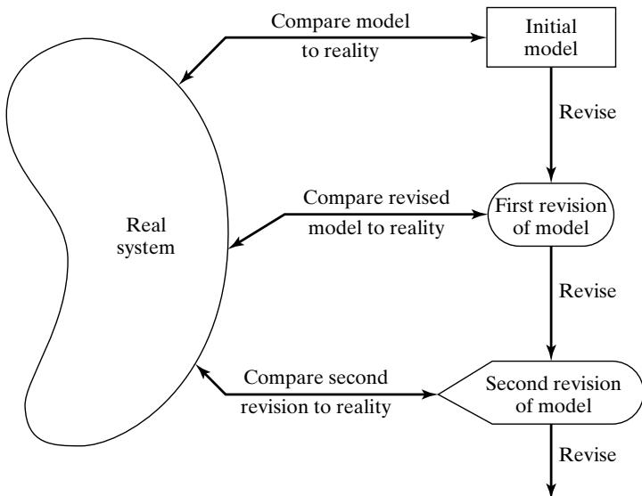 Figure 3 Iterative process of calibrating a model.
Validation is not an either/or proposition—no model is ever totally representative of the system under study. In addition, each revision of the model, as pictured in Figure 3, involves some cost, time, and effort. The modeler must weigh the possible, but not guaranteed, increase in model accuracy versus the cost of increased validation effort. Usually, the modeler (and model users) have some maximum discrepancy between model predictions and system behavior that would be acceptable. If this level of accuracy cannot be obtained within the budget constraints, either expectations of mode accuracy must be lowered, or the model must be abandoned.
As an aid in the validation process, Naylor and Finger [1967] formulated a three-step approach that has been widely followed:
Step 1. Build a model that has high face validity.
Step 2. Validate model assumptions.
Step 3. Compare the model input-output transformations to corresponding input-output transformations for the real system.
The next five subsections investigate these three steps in detail.
3.1 Face Validity
The first goal of the simulation modeler is to construct a model that appears reasonable on its face to model users and others who are knowledgeable about the real system being simulated. The potentia users of a model should be involved in model construction from its conceptualization to its implementation, to ensure that a high degree of realism is built into the model through reasonable assumptions regarding system structure and through reliable data. Potential users and knowledgeable people can also evaluate model output for reasonableness and can aid in identifying model deficiencies. Thus, the users can be involved in the calibration process as the model is improved iteratively by the insights gained from identification of the initial model deficiencies. Another advantage of user involvement is the increase in the model’s perceived validity, or credibility, without which a manager would no be willing to trust simulation results as a basis for decision making.
Sensitivity analysis can also be used to check a model’s face validity. The model user is asked whether the model behaves in the expected way when one or more input variables is changed. For example, in most queueing systems, if the arrival rate of customers (or demands for service) were to increase, it would be expected that utilizations of servers, lengths of lines, and delays would tend to increase (although by how much might well be unknown). From experience and from observations on the real system (or similar related systems), the model user and model builder would probably have some notion at least of the direction of change in model output when an input variable is increased or decreased. For most large-scale simulation models, there are many input variables and thus many possible sensitivity tests. The model builder must attempt to choose the most critical input variables for testing if it is too expensive or time consuming to vary all input variables. If real system data are available for at least two settings of the input parameters, objective scientific sensitivity tests can be conducted via appropriate statistical techniques.
3.2 Validation of Model Assumptions
Model assumptions fall into two general classes: structural assumptions and data assumptions. Structural assumptions involve questions of how the system operates and usually involve simplifications and abstractions of reality. For example, consider the customer queueing and service facility in a bank. Customers can form one line, or there can be an individual line for each teller. If there are many lines, customers could be served strictly on a first-come-first-served basis, or some customers could change lines if one line is moving faster. The number of tellers could be fixed or variable. These structural assumptions should be verified by actual observation during appropriate time periods and by discussions with managers and tellers regarding bank policies and actual implementation of these policies.
Data assumptions should be based on the collection ofreliable data and correct statistical analysis of the data. For example, in the bank study previously mentioned, data were collected on
interarrival times of customers during several 2-hour periods of peak loading (“rush-hour” traffic);
interarrival times during a slack period;
service times for commercial accounts;
service times for personal accounts.
The reliability of the data was verified by consultation with bank managers, who identified typica rush hours and typical slack times. When combining two or more data sets collected at differen times, data reliability can be further enhanced by objective statistical tests for homogeneity of data. (Do two data sets X and Y on service times for personal accounts, collected at two differen times, come from the same parent population? If so, the two sets can be combined.) Additional tests might be required, to test for correlation in the data. As soon as the analyst is assured of dealing with a random sample (i.e., correlation is not present), the statistical analysis can begin.
Whether done manually or by special-purpose software, the analysis consists of three steps:
Step 1. Identify an appropriate probability distribution.
Step 2. Estimate the parameters of the hypothesized distribution.
Step 3. Validate the assumed statistical model by a goodness-of-fit test, such as the chi-square or Kolmogorov–Smirnov test, and by graphical methods.
The use of goodness-of-fit tests is an important part of the validation of data assumptions.
3.3 Validating Input-Output Transformations
The ultimate test of a model, and in fact the only objective test of the model as a whole, is the model’s ability to predict the future behavior of the real system when the model input data match the rea inputs and when a policy implemented in the model is implemented at some point in the system. Furthermore, if the level of some input variables (e.g., the arrival rate of customers to a service facility) were to increase or decrease, the model should accurately predict what would happen in the real system under similar circumstances. In other words, the structure of the model should be accurate enough for the model to make good predictions, not just for one input data set, but for the range of input data sets that are of interest.
In this phase of the validation process, the model is viewed as an input-output transformation— that is, the model accepts values of the input parameters and transforms these inputs into outpu measures of performance. It is this correspondence that is being validated.
Instead ofvalidating the model input-output transformations by predicting the future, the modeler could use historical data that have been reserved for validation purposes only—that is, if one data set has been used to develop and calibrate the model, it is recommended that a separate data set be used as the final validation test. Thus, accurate “prediction of the past” can replace prediction of the future for the purpose of validating the model.
A model is usually developed with primary interest in a specific set of system responses to be measured under some range of input conditions. For example, in a queueing system, the responses may be server utilization and customer delay, and the range of input conditions (or input variables) may include two or three servers at some station and a choice of scheduling rules. In a production system, the response may be throughput (i.e., production per hour), and the input conditions may be a choice of several machines that run at different speeds, with each machine having its own breakdown and maintenance characteristics.
In any case, the modeler should use the main responses of interest as the primary criteria for validating a model. If the model is used later for a purpose different from its original purpose, the model should be revalidated in terms of the new responses of interest and under the possibly new input conditions.
A necessary condition for the validation of input-output transformations is that some version of the system under study exist, so that system data under at least one set of input conditions can be collected to compare to model predictions. If the system is in the planning stages and no system operating data can be collected, complete input-output validation is not possible. Other types o validation should be conducted, to the extent possible. In some cases, subsystems of the planned system may exist, and a partial input-output validation can be conducted.
Presumably, the model will be used to compare alternative system designs or to investigate system behavior under a range of new input conditions. Assume for now that some version of the system is operating and that the model of the existing system has been validated. What, then, can be said about the validity of the model when different inputs are used? That is, if model inputs are being changed to represent a new system design, or a new way to operate the system, or even hypothesized future conditions, what can be said about the validity of the model with respect to this new bu nonexistent proposed system or to the system under new input conditions?
First, the responses of the two models under similar input conditions will be used as the criteria for comparison of the existing system to the proposed system. Validation increases the modeler’s confidence that the model of the existing system is accurate. Second, in many cases, the proposed system is a modification of the existing system, and the modeler hopes that confidence in the mode of the existing system can be transferred to the model of the new system. This transfer of confidence usually can be justified if the new model is a relatively minor modification of the old model in terms of changes to the operational model (it may be a major change for the actual system). Changes in the operational model ranging from relatively minor to relatively major include the following:
minor changes of single numerical parameters, such as the speed of a machine, the arrival rate of customers (with no change in distributional form of interarrival times), the number of servers in a parallel service center, or the mean time to failure or mean time to repair of a machine;
minor changes in the form of a statistical distribution, such as the distribution of a service time or a time to failure of a machine;
major changes in the logical structure of a subsystem, such as a change in queue discipline for a waiting-line model or a change in the scheduling rule for a job-shop model;
major changes involving a different design for the new system, such as a computerized inventory control system replacing an older noncomputerized system, or an automated storageand-retrieval system replacing a warehouse system in which workers manually pick items using fork trucks.
If the change to the operational model is minor, such as in items 1 or 2, these changes can be carefully verified and output from the new model accepted with considerable confidence. If a sufficiently similar subsystem exists elsewhere, it might be possible to validate the submodel tha represents the subsystem and then to integrate this submodel with other validated submodels to build a complete model. In this way, partial validation of the substantial model changes in items 3 and 4 might be possible. Unfortunately, there is no way to validate the input-output transformations of a model of a nonexisting system completely. In any case, within time and budget constraints, the modeler should use as many validation techniques as possible, including input-output validation o subsystem models if operating data can be collected on such subsystems.
Example 2 will illustrate some of the techniques that are possible for input-output validation and will discuss the concepts of an input variable, uncontrollable variable, decision variable, outpu or response variable, and input-output transformation in more detail.
Example 2: The Fifth National Bank of Jaspar
The Fifth National Bank of Jaspar, as shown in Figure 4, is planning to expand its drive-in service at the corner of Main Street. Currently. there is one drive-in window serviced by one teller. Only one or two transactions are allowed at the drive-in window, so it was assumed that each service time was a random sample from some underlying population. Service times and interarrival times were collected for the 90 customers who arrived between 11:00 A.M. and 1:00 P.M. on a Friday. This time slot was selected for data collection after consultation with management and the teller because it was felt to be representative of a typical rush hour.
Data analysis led to the conclusion that arrivals could be modeled as a Poisson process at a rate of 45 customers per hour and that service times were approximately normally distributed, with mean
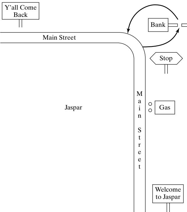 Figure 4 Drive-in window at the Fifth National Bank.
1.1 minutes and standard deviation 0.2 minute. Thus, the model has two input variables:
interarrival times, exponentially distributed (i.e., a Poisson arrival process) at rate per hour;
service times, assumed to be Each input variable has a level: the rate per hour for the interarrival times, and the mean 1.1 minutes and standard deviation 0.2 minute for the service times. The interarrival times are examples of uncontrollable variables (i.e., uncontrollable by management in the real system). The service times are also treated as uncontrollable variables, although the level of the service times might be partially controllable. If the mean service time could be decreased to 0.9 minute by installing a computer terminal, the level of the service-time variable becomes a decision variable or controllable parameter. Setting all decision variables at some level constitutes a policy. For example, the curren bank policy is one teller , mean service time minutes, and one line for waiting cars are used to denote decision variables.) Decision variables are under management’s control; the uncontrollable variables, such as arrival rate and actual arrival times, are not under management’s control. The arrival rate might change from time to time, but such change is treated as being due to external factors not under management control.
Table 1 Input and Output Variables for Model of Current Bank Operations
| Input Variables | Model Output Variables, Y |
|---|---|
| D = decision variables | Variables of primary interest to management (Y1, Y2, Y3) |
| X = other variables | |
| Y1 = teller's utilization | |
| Poisson arrivals at rate = 45/hour | Y2 = average delay |
| X11, X12, … | Y3 = maximum line length |
| Service times, N(D2, 0.22) | Other output variables of secondary interest |
| X21, X22, … | |
| Y4 = observed arrival rate | |
| D1 = 1 (one teller) | Y5 = average service time |
| D2 = 1.1 minutes (mean service time) | Y6 = sample standard deviation of service times |
| D3 = 1 (one line) | |
| Y7 = average length of waiting line |
A model of current bank operations was developed and verified in close consultation with bank management and employees. Model assumptions were validated, as discussed in Section 3.2. The resulting model is now viewed as a “black box” that takes all input-variable specifications and transforms them into a set of output or response variables. The output variables consist of all statistics of interest generated by the simulation about the model’s behavior. For example, management is interested in the teller’s utilization at the drive-in window (percent of time the teller is busy at the window), average delay in minutes of a customer from arrival to beginning of service, and the maximum length of the line during the rush hour. These input and output variables are shown in Figure 5 and are listed in Table 1, together with some additional output variables. The uncontrollable input variables are denoted by X, the decision variables by D, and the output variables by Y. From the “black box” point of view, the model takes the inputs X and D and produces the outputs namely
or
Here f denotes the transformation that is due to the structure of the model. For the Fifth Nationa Bank study, the exponentially distributed interarrival time generated in the model between customer and customer n is denoted by . (Do not confuse with ; the latter was an observation made on the real system.) The normally distributed service time generated in the model for customer n is denoted by . The set of decision variables, or policy, is ) for current operations. The output, or response, variables are denoted by and are defined in Table 1.
For validation of the input-output transformations of the bank model to be possible, real system data must be available, comparable to at least some of the model output Y of Table 1. The system responses should have been collected during the same time period (from 11:00 A.M. to 1:00 P.M. on the same Friday) in which the input data were collected. This is important because, if system response data were collected on a slower day (say, an arrival rate of 40 per hour), the system responses such as teller utilization , average delay , and maximum line length would be expected to be lower than the same variables during a time slot when the arrival rate was 45 per hour, as observed. Suppose that the delay of successive customers was measured on the same Friday between 11:00 A.M. and 1:00 P.M. and that the average delay was found to be minutes. For the purpose of validation, we will consider this to be the true mean value 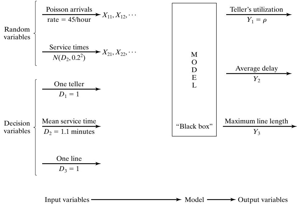 Figure 5 Model input-output transformation.
When the model is run with generated random variates and , it is expected that observed values of average delay should be close to minutes. The generated input values and cannot be expected to replicate the actual input values and of the real system exactly, but they are expected to replicate the statistical pattern of the actual inputs. Hence, simulation-generated values of are expected to be consistent with the observed system variable minutes. Now consider how the modeler might test this consistency.
The modeler makes a small number of statistically independent replications of the model. Statistical independence is guaranteed by using nonoverlapping sets of random numbers produced by the random-number generator or by choosing seeds for each replication independently (from a random number table). The results of six independent replications, each of 2 hours duration, are given in Table 2.
Observed arrival rate and sample average service time for each replication of the model are also noted, to be compared with the specified values of 45/hour and 1.1 minutes, respectively. The validation test consists of comparing the system response, namely average delay minutes, to the model responses . Formally, a statistical test of the null hypothesis
versus
is conducted. If is not rejected, then, on the basis of this test, there is no reason to consider the model invalid. If is rejected, the current version of the model is rejected, and the modeler is forced to seek ways to improve the model, as illustrated by Figure 3. As formulated here, the appropriate statistical test is the t test, which is conducted in the following manner:
Choose a level of significance α and a sample size n. For the bank model, choose
Compute the sample mean and the sample standard deviation S over the n replications, by using:
and
where , are as shown in Table 2.
Get the critical value of t from Table A.5 in the Appendix. For a two-sided test, such as that in equation (1), use for a one-sided test, use , as appropriate (n 1 being the degrees of freedom). From Table for a two-sided test.
Table 2 Results of Six Replications of the Bank Model
| Replication | (arrivals/hour) | (minutes) | $ Y_2 = Average Delay $(minutes) |
|---|---|---|---|
| 1 | 51 | 1.07 | 2.79 |
| 2 | 40 | 1.12 | 1.12 |
| 3 | 45.5 | 1.06 | 2.24 |
| 4 | 50.5 | 1.10 | 3.45 |
| 5 | 53 | 1.09 | 3.13 |
| 6 | 49 | 1.07 | 2.38 |
| Sample mean | 2.51 | ||
| Standard deviation | 0.82 |
Compute the test statistic
where is the specified value in the null hypothesis . Here minutes, so that
For the two-sided test,$\mathrm{i f} \left| t_{0} \right| > t_{\alpha / 2 , n - 1} ,$, reject . Otherwise, do not reject . [For the one-sided test with , reject if with , reject if Since $| t | = 5 . 34 > t_{0 . 025 , 5} = 2 . 571 $, reject , and conclude that the model is inadequate in its prediction of average customer delay.
Recall that, in the testing of hypotheses, rejection of the null hypothesis is a strong conclusion, because
and the level of significance α is chosen small, say , as was done here. Equation says that the probability is low of making the error of rejecting when is in fact true —that is, the probability is small of declaring the model invalid when it is valid (with respect to the variable being tested). The assumptions justifying a t test are that the observations are normally and independently distributed. Are these assumptions met in the present case?
The ith observation is the average delay of all drive-in customers who began service during the ith simulation run of 2 hours; thus, by a Central Limit Theorem effect, it is reasonable to assume that each observation is approximately normally distributed, provided that the number of customers it is based on is not too small.
The observations , are statistically independent by design—that is, by choosing the random-number seeds independently for each replication or by using nonoverlapping streams.
The t statistic computed by Equation (2) is a robust statistic—that is, it is distributed approximately as the t distribution with n 1 degrees of freedom, even when . are not exactly normally distributed, and thus the critical values in Table A.5 can reliably be used.
Now that the model of the Fifth National Bank of Jaspar has been found lacking, what should the modeler do? Upon further investigation, the modeler realized that the model contained two unstated assumptions:
When a car arrived to find the window immediately available, the teller began service immediately.
There is no delay between one service ending and the next beginning, when a car is waiting.
Assumption 2 was found to be approximately correct, because a service time was considered to begin when the teller actually began service but was not considered to have ended until the car had exited the drive-in window and the next car, if any, had begun service, or the teller saw that the line was empty. On the other hand, assumption 1 was found to be incorrect because the teller had other duties—mainly, serving walk-in customers if no cars were present—and tellers always finished with a previous customer before beginning service on a car. It was found that walk-in customers were always present during rush hour; that the transactions were mostly commercial in nature, taking a considerably longer time than the time required to service drive-up customers; and that, when an arriving car found no other cars at the window, it had to wait until the teller finished with the presen walk-in customer. To correct this model inadequacy, the structure of the model was changed to include the additional demand on the teller’s time, and data were collected on service times of walkin customers. Analysis of these data found that they were approximately exponentially distributed with a mean of 3 minutes.
The revised model was run, yielding the results in Table 3. A test of the null hypothesis minutes was again conducted, according to the procedure previously outlined.
Choose and (sample size).
Compute minutes, minutes.
Look in Table A.5, the critical value Compute the test statistic Since $| t_{0} | < t_{0 . 025 , 5} = 2 . 571 $, do not reject , and thus tentatively accept the model as valid.
Failure to reject must be considered as a weak conclusion unless the power of the test has been estimated and found to be high (close to 1)—that is, it can be concluded only that the data at hand were not sufficient to reject the hypothesis minutes. In other words, this test detects no inconsistency between the sample data and the specified mean The power of a test is the probability of detecting a departure from when, in fact, such a departure exists. In the validation context, the power of the test is the probability of detecting an invalid model. The power may also be expressed as 1 minus the probability of a Type II, or error, where to reject $ H_{0} | H_{1}$ is true) is the probability of accepting the model as valid when it is not valid.
Table 3 Results of Six Replications of the Revised Bank Model
| Replication | (arrivals/hour) | (minutes) | $ Y_2 = Average Delay $(minutes) |
|---|---|---|---|
| 1 | 51 | 1.07 | 5.37 |
| 2 | 40 | 1.11 | 1.98 |
| 3 | 45.5 | 1.06 | 5.29 |
| 4 | 50.5 | 1.09 | 3.82 |
| 5 | 53 | 1.08 | 6.74 |
| 6 | 49 | 1.08 | 5.49 |
| Sample mean | 4.78 | ||
| Standard deviation | 1.66 |
To consider failure to reject as a strong conclusion, the modeler would want to be small. Now, depends on the sample size n and on the true difference between and minutes—that is, on
where the population standard deviation of an individual , is estimated by S. Tables A.10 and A.11 are typical operating-characteristic (OC) curves, which are graphs of the probability of a Type II error versus δ for given sample size n. Table A.10 is for a two-sided t test; Table A.11 is for a one-sided t test. Suppose that the modeler would like to reject (model validity) with probability at least 0.90 if the true mean delay of the model,, differed from the average delay in the system, minutes, by 1 minute. Then δ is estimated by
For the two-sided test with , use of Table A.10 results in
To guarantee that , as was desired by the modeler, Table A.10 reveals that a sample size of approximately independent replications would be required—that is, for a sample size 6 and assuming that the population standard deviation is 1.66, the probability of accepting (mode validity), when, in fact, the model is invalid $( | E ( Y_{2} ) - \mu_{0} | = 1 $ minute), is , which is quite high. If a 1-minute difference is critical, and if the modeler wants to control the risk of declaring the model valid when model predictions are as much as 1 minute off, a sample size of replications is required to achieve a power of 0.9. If this sample size is too high, either a higher risk (lower power) or a larger difference δ must be considered.
In general, it is always best to control the Type II error, or error, by specifying a critica difference δ and choosing a sample size by making use of an appropriate OC curve. (Computation of power and use of OC curves for a wide range of tests is discussed in Hines, Montgomery, Goldsman, and Borror [2002].) In summary, in the context of model validation, the Type I error is the rejection of a valid model and is easily controlled by specifying a small level of significance α, say,0.05, or 0.01. The Type II error is the acceptance of a model as valid when it is invalid. For a fixed sample size n, increasing α will decrease , the probability of a Type II error. Once α is set, and the critical difference to be detected is selected, the only way to decrease is to increase the sample size. A Type II error is the more serious of the two types of errors; thus, it is important to design the simulation experiments to control the risk of accepting an invalid model. The two types of error are summarized in Table 4, which compares statistical terminology to modeling terminology.
Note that validation is not to be viewed as an either/or proposition, but rather should be viewed in the context of calibrating a model, as conceptually exhibited in Figure 3. If the current version of the bank model produces estimates of average delay that are not close enough to real system behavior , the source of the discrepancy is sought, and the model is revised in light of this new knowledge. This iterative scheme is repeated until model accuracy is judged adequate.
Table 4 Types of Error in Model Validation
| Statistical Terminology | Modeling Terminology | Associated Risk |
|---|---|---|
| Type I: rejecting when is true | Rejecting a valid model | |
| Type II: failure to reject when is true | Failure to reject an invalid model |
Philosophically, the hypothesis-testing approach tries to evaluate whether the simulation and the real system are the same with respect to some output performance measure or measures. A different, but closely related, approach is to attempt to evaluate whether the simulation and the real-system performance measures are close enough by using confidence intervals.
We continue to assume that there is a known output performance measure for the existing system, denoted by , and an unknown performance measure of the simulation,, that we hope is close. The hypothesis-testing formulation tested whether the confidence-interval formulation tries to bound the difference $| \mu - \mu_{0} |$ to see whether it is , a difference that is small enough to allow valid decisions to be based on the simulation. The value of ε is set by the analyst.
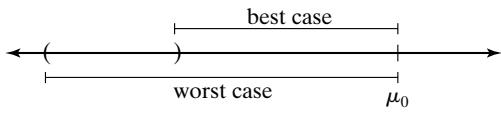
Specifically, if is the simulation output and , then we execute the simulation and form a confidence interval for , such as . The determination of whether to accep the model as valid or to refine the model depends on the best-case and worst-case error implied by the confidence interval.
- Suppose the confidence interval does not contain . [See Figure 6(a).]
(a) If the best-case error is then the difference in performance is large enough, even in the best case, to indicate that we need to refine the simulation model.
(b) If the worst-case error i , then we can accept the simulation model as close enough to be considered valid.
(c) If the best-case error is , but the worst-case error is then additional simulation replications are necessary to shrink the confidence interval until a conclusion can be reached.
- Suppose the confidence interval does contain . [See Figure (a) If either the best-case or worst-case error is then additional simulation replications are necessary to shrink the confidence interval until a conclusion can be reached.
(b) If the worst-case error , then we can accept the simulation model as close enough to be considered valid.
In Example minutes, and “close enough” was minute of expected customer delay. A 95% confidence interval, based on the 6 replications in Table 2, is
 (a)
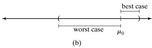 Figure 6 Validation of the input-output transformation (a) when the known value falls outside, and (b) when the known value falls inside, the confidence interval.
yielding the interval [1.65, 3.37]. As in Figure 6(a), falls outside the confidence interval. Since in the best case $| 3 . 37 - 4 . 3 | = 0 . 93 < 1 $, but in the worst case $| 1 . 65 - 4 . 3 | = 2 . 65 > 1 $ additional replications are needed to reach a decision.
3.4 Input-Output Validation: Using Historical Input Data
When using artificially generated data as input data, as was done to test the validity of the bank models in Section 3.3, the modeler expects the model to produce event patterns that are compatible with, but not identical to, the event patterns that occurred in the real system during the period of data collection. Thus, in the bank model, artificial input data for interarriva and service times were generated, and replicates of the output data were compared to what was observed in the real system by means of the hypothesis test stated in equation (1). An alternative to generating input data is to use the actual historical record,, to drive the simulation model and then to compare model output with system data.
To implement this technique for the bank model, the data . and . would have to be entered into the model into arrays, or stored in a file to be read as the need arose. Just after customer n arrived at time , customer n 1 would be scheduled on the future event list to arrive at future time (without any random numbers being generated). If customer n were to begin service at time , a service completion would be scheduled to occur at time This event scheduling without random-number generation could be implemented quite easily in a general-purpose programming language or most simulation languages by using arrays to store the data or reading the data from a file.
When using this technique, the modeler hopes that the simulation will duplicate as closely as possible the important events that occurred in the real system. In the model of the Fifth National Bank of Jaspar, the arrival times and service durations will exactly duplicate what happened in the rea system on that Friday between 11:00 A.M. and 1:00 P.M. If the model is sufficiently accurate, then the delays of customers, lengths of lines, utilizations of servers, and departure times of customers predicted by the model will be close to what actually happened in the real system. It is, of course, the model-builder’s and model-user’s judgment that determines the level of accuracy required.
To conduct a validation test using historical input data, it is important that all the input data and all the system response data, such as average delay , be collected during the same time period. Otherwise, the comparison of model responses to system responses, such as the comparison of average delay in the model to that in the system , could be misleading. The responses and depend both on the inputs and and on the structure of the system (or model). Implementation of this technique could be difficult for a large system, because of the need for simultaneous data collection of all input variables and those response variables of primary interest. In some systems, electronic counters and devices are used to ease the data-collection task by automatically recording certain types of data. The following example was based on two simulation models reported in Carson et al. [1981a, b], in which simultaneous data collection and the subsequen validation were both completed successfully.
Example 3: The Candy Factory
The production line at the Sweet Lil’ Things Candy Factory in Decatur consists of three machines that make, package, and box their famous candy. One machine (the candy maker) makes and wraps individual pieces of candy and sends them by conveyor to the packer. The second machine (the packer) packs the individual pieces into a box. A third machine (the box maker) forms the boxes and supplies them by conveyor to the packer. The system is illustrated in Figure 7.
Each machine is subject to random breakdowns due to jams and other causes. These breakdowns cause the conveyor to begin to empty or fill. The conveyors between the two makers and the packer are used as a temporary storage buffer for in-process inventory. In addition to the randomly occurring breakdowns, if the candy conveyor empties, a packer runtime is interrupted and the packer remains idle until more candy is produced. If the box conveyor empties because of a long random breakdown of the box machine, an operator manually places racks of boxes onto the packing machine. If a conveyor fills, the corresponding maker becomes idle. The purpose of the model is to investigate the frequency of those operator interventions that require manual loading of racks of boxes as a function of various combinations of individual machines and lengths of conveyor. Different machines have different production speeds and breakdown characteristics, and longer conveyors can hold more inprocess inventory. The goal is to hold operator interventions to an acceptable level while maximizing production. Machine stoppages (whether due to a full or an empty conveyor) cause damage to the product, so this is also a factor in production.
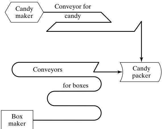 Figure 7 Production line at the candy factory.
A simulation model of the candy factory was developed, and a validation effort using historical inputs was conducted. Engineers in the candy factory set aside a 4-hour time slot from 7:00 A.M. to 11:00 A.M. to collect data on an existing production line. For each machine—say, machine i—time to failure and downtime duration
were collected. For machine is the jth runtime (or time to failure), and is the successive downtime. A runtime can be interrupted by a full or empty conveyor (as appropriate), but resumes when conditions are right. Initial system conditions at 7:00 A.M. were recorded so that they could be duplicated in the model as initial conditions at time 0. Additionally, system responses of primary interest—the production level , and the number and time of occurrence of operator interventions—were recorded for comparison with model predictions.
The system input data and were fed into the model and used as runtimes and random downtimes. The structure of the model determined the occurrence of shutdowns due to a full or empty conveyor and the occurrence of operator interventions. Model response variables were collected for comparison to the corresponding system response variables The closeness of model predictions to system performance aided the engineering staff considerably in convincing management of the validity of the model. These results are shown in Table 5. A simple display such as Table 5 can be quite effective in convincing skeptical engineers and managers of a model’s validity—perhaps more effectively than the most sophisticated statistical methods!
With only one set of historical input and output data, only one set of simulated output data can be obtained, and thus no simple statistical tests based on summary measures are possible. However, if K historical input data sets are collected, and K observations of some system response variable are collected, such that the output measure corresponds to thejth input set, an objective statistical test becomes possible. For example, could be the average delay of all customers who were served during the time the jth input data set was collected. With the K input data sets in hand, the modeler now runs the model K times, once for each input set, and observes the simulated results corresponding to . Continuing the same example, would be the average delay predicted by the model for the jth input set. The data available for comparison appears as in Table 6.
Table 5 Validation of the Candy-Factory Model
| Response i | System | Model |
|---|---|---|
| 1. Production level | 897,208 | 883,150 |
| 2. Number of operator interventions | 3 | 3 |
| 3. Time of occurrence | 7:22, 8:41, 10:10 | 7:24, 8:42, 10:14 |
Table 6 Comparison of System and Model Output Measures for Identical Historical Inputs
| Input Data Set | System Output | Model Output | Observed Difference | Squared Deviation from Mean |
|---|---|---|---|---|
| 1 | ||||
| 2 | ||||
| 3 | ||||
| . | . | . | . | . |
| . | . | . | . | . |
| . | . | . | . | . |
| K | ||||
If the K input data sets are fairly homogeneous, it is reasonable to assume that the K observed differences , are identically distributed. Furthermore, if the collection o the K sets of input data was separated in time—say, on different days—it is reasonable to assume tha the K differences are statistically independent and, hence, that the differences constitute a random sample. In many cases, each and is a sample average over customers, and so (by the Central Limit Theorem) the differences are approximately normally distributed with some mean and variance . The appropriate statistical test is then a t test of the null hypothesis of no mean difference:
versus the alternative of significant difference:
The proper test is a paired t test is paired with , each having been produced by the first input data set, and so on). First, compute the sample mean difference, d¯ , and the sample variance,, by the formulas given in Table 6. Then, compute the t statistic as
(with , and get the critical value from Table A.5, where α is the prespecified significance level and is the number of degrees of freedom. If $| t_{0} | > t_{\alpha / 2 , K - 1} ,$, reject the hypothesis of no mean difference, and conclude that the model is inadequate. If t do not reject , and hence conclude that this test provides no evidence of model inadequacy.
Engineers at the Sweet Lil’ Things Candy Factory decided to expand the initial validation effort reported in Example 3. Electronic devices were installed that could automatically monitor one of the production lines, and the validation effort of Example 3 was repeated with K 5 sets of input data. The system and the model were compared on the basis of production level. The results are shown in Table 7.
A paired t test was conducted to test , or equivalently,, where is the system production level and is the production level predicted by the simulated model. Let the level of significance be . Using the results in Table 7, the test statistic, as given by equation (4), is
From Table A.5, the critical value is . Since $| t_{0} | = 1 . 37 < t_{0 . 025 , 4} =$2.78, the null hypothesis cannot be rejected on the basis of this test—that is, no inconsistency is detected between system response and model predictions in terms of mean production level. If had been rejected, the modeler would have searched for the cause of the discrepancy and revised the model, in the spirit of Figure 3.
Table 7 Validation of the Candy-Factory Model (cont.)
| Input Data Set j | System Production | Model Production | Observed Difference | Squared Deviation from Mean |
|---|---|---|---|---|
| 1 | 897,208 | 883,150 | 14,058 | |
| 2 | 629,126 | 630,550 | -1,424 | |
| 3 | 735,229 | 741,420 | -6,191 | |
| 4 | 797,263 | 788,230 | 9,033 | |
| 5 | 825,430 | 814,190 | 11,240 | |
3.5 Input-Output Validation: Using a Turing Test
In addition to statistical tests, or when no statistical test is readily applicable, personnel knowledgeable about system behavior can be used to compare model output to system output. For example, suppose that five reports of system performance over five different days are prepared, and simulation outpu data are used to produce five “fake” reports. The 10 reports should all be in exactly the same forma and should contain information of the type that managers and engineers have previously seen on the system. The 10 reports are randomly shuffled and given to the engineer, who is asked to decide which reports are fake and which are real. If the engineer identifies a substantial number of the fake reports, the model builder questions the engineer and uses the information gained to improve the model. If the engineer cannot distinguish between fake and real reports with any consistency, the modeler will conclude that this test provides no evidence of model inadequacy. For further discussion and an application to a real simulation, the reader is referred to Schruben [1980]. This type of validation test is commonly called a Turing test. Its use as model development proceeds can be a valuable tool in detecting model inadequacies and, eventually, in increasing model credibility as the model is improved and refined.
4 Summary
Validation of simulation models is of great importance. Decisions are made on the basis of simulation results; thus, the accuracy of these results should be subject to question and investigation.
Quite often, simulations appear realistic on the surface because simulation models, unlike analytic models, can incorporate any level of detail about the real system. To avoid being “fooled” by this apparent realism, it is best to compare system data to model data and to make the comparison by using a wide variety of techniques, including an objective statistical test, if at all possible.
As discussed by Van Horn [1969, 1971], some of the possible validation techniques, in order of increasing cost-to-value ratios, include
Develop models with high face validity by consulting people knowledgeable about system behavior on model structure, model input, and model output. Use any existing knowledge in the form of previous research and studies, observation, and experience.
Conduct simple statistical tests of input data for homogeneity, for randomness, and for goodness of fit to assumed distributional forms.
Conduct a Turing test. Have knowledgeable people (engineers, managers) compare mode output to system output and attempt to detect the difference.
Compare model output to system output by means of statistical tests.
After model development, collect new system data and repeat techniques 2 to 4.
Build the new system (or redesign the old one), conforming to the simulation results, collec data on the new system, and use the data to validate the model (not recommended if this is the only technique used).
Do little or no validation. Implement simulation results without validating. (Not recommended.)
It is usually too difficult, too expensive, or too time consuming to use all possible validation techniques for every model that is developed. It is an important part of the model-builder’s task to choose those validation techniques most appropriate, both to assure model accuracy and to promote model credibility.
REFERENCES
BALCI, O. [1994], “Validation, Verification and Testing Techniques throughout the Life Cycle of a Simulation Study,” Annals ofOperations Research, Vol. 53, pp. 121–174.
BALCI, O. [1998], “Verification, Validation, and Testing,” in Handbook ofSimulation, J. Banks, ed., John Wiley, New York.
BALCI, O. [2003], “Verification, Validation, and Certification of Modeling and Simulation Applications,” in Proceedings ofthe 2003 Winter Simulation Conference, S. Chick, P. J. S´anchez, D. Ferrin, and D. J. Morrice, eds., New Orleans, LA, Dec. 7–10, pp. 150–158.
BALCI, O.,AND R. G. SARGENT [1982a], “Some Examples ofSimulation ModelValidation Using Hypothesis Testing,” in Proceedings of the 1982 Winter Simulation Conference, H. J. Highland, Y. W. Chao, and O. S. Madrigal, eds., San Diego, CA, Dec. 6–8, pp. 620–629.
BALCI, O., AND R. G. SARGENT [1982b], “Validation of Multivariate Response Models Using Hotelling’s Two-Sample T^2 Test,” Simulation, Vol. 39, No. 6, pp. 185–192.
BALCI, O., AND R. G. SARGENT [1984a], “Validation of Simulation Models via Simultaneous Confidence Intervals,” American Journal ofMathematical Management Sciences, Vol. 4, Nos. 3 & 4, pp. 375–406.
BALCI, O., AND R. G. SARGENT [1984b], “A Bibliography on the Credibility Assessment and Validation of Simulation and Mathematical Models,” Simuletter, Vol. 15, No. 3, pp. 15–27.
BORTSCHELLER, B. J., AND E. T. SAULNIER [1992], “Model Reusability in a Graphical Simulation Package,” in Proceedings ofthe 24th Winter Simulation Conference, J. J. Swain, D. Goldsman, R. C. Crain, and J. R. Wilson, eds., Arlington, VA, Dec. 13–16, pp. 764–772.
CARSON, J. S., [1986], “Convincing Users of Model’s Validity is Challenging Aspect of Modeler’s Job,” Industrial Engineering, June, pp. 76–85.
CARSON, J. S. [2002], “Model Verification and Validation,” in Proceedings of the 34th Winter Simulation Conference, E. Y¨ucesan, C.-H. Chen, J. L. Snowdon, and J. M. Charnes, eds., San Diego, Dec. 8-11, pp. 52–58.
CARSON, J. S., N. WILSON, D. CARROLL, AND C. H. WYSOWSKI [1981a], “A Discrete Simulation Model of a Cigarette Fabrication Process,” Proceedings ofthe Twelfth Modeling and Simulation Conference, University of Pittsburgh, PA., Apr. 30–May 1, pp. 683–689.
CARSON, J. S., N. WILSON, D. CARROLL, AND C. H. WYSOWSKI [1981b], “Simulation of a Filter Rod Manufacturing Process,” Proceedings ofthe 1981 Winter Simulation Conference, T. I. Oren, C. M. Delfosse, and C. M. Shub, eds., Atlanta, GA, Dec. 9–11, pp. 535–541.
GAFARIAN, A. V., AND J. E. WALSH [1970], “Methods for Statistical Validation of a Simulation Model fo Freeway Traffic near an On-Ramp,” Transportation Research, Vol. 4, p. 379–384
GASS, S. I. [1983], “Decision-Aiding Models: Validation, Assessment, and Related Issues for Policy Analysis,” Operations Research, Vol. 31, No. 4, pp. 601–663.
HINES, W. W., D. C. MONTGOMERY, D. M. GOLDSMAN, AND C. M. BORROR [2002], Probability and Statistics in Engineering, 4th ed., Wiley, New York.
KLEIJNEN, J. P. C. [1987], Statistical Toolsfor Simulation Practitioners, Marcel Dekker, New York.
KLEIJNEN, J. P. C. [1993], “Simulation and Optimization in Production Planning: A Case Study,” Decision Support Systems, Vol. 9, pp. 269–280.
KLEIJNEN, J. P. C. [1995], “Theory and Methodology: Verification and Validation of Simulation Models,” European Journal ofOperational Research, Vol. 82, No. 1, pp. 145–162.
LAW, A. M., AND W. D. KELTON [2000], Simulation Modeling andAnalysis, 3d ed., McGraw-Hill, NewYork.
NAYLOR, T. H., AND J. M. FINGER [1967], “Verification of Computer Simulation Models,” Management Science, Vol. 2, pp. B92–B101.
OREN, T. [1981], “Concepts and Criteria to Assess Acceptability of Simulation Studies: A Frame of Reference,” Communications ofthe Associationfor Computing Machinery, Vol. 24, No. 4, pp. 180–189.
SARGENT, R. G. [2003], “Verification and Validation of Simulation Models,” in Proceedings of the 2003 Winter Simulation Conference, S. Chick, P. J. S´anchez, D. Ferrin, and D. J. Morrice, eds., New Orleans, LA, Dec. 7–10, pp. 37–48.
SCHECTER, M., AND R. C. LUCAS [1980], “Validating a Large Scale Simulation Model of Wilderness Recreation Travel,” Interfaces, Vol. 10, pp. 11–18.
SCHRUBEN, L. W. [1980], “Establishing the Credibility of Simulations,” Simulation, Vol. 34, pp. 101–105.
SHANNON, R. E. [1975], Systems Simulation: The Art and Science. Prentice-Hall, Englewood Cliffs, NJ.
VAN HORN, R. L. [1969], “Validation,” in The Design ofComputer Simulation Experiments, T. H. Naylor, ed., pp. 232–235 Duke University Press, Durham, NC
VAN HORN, R. L. [1971], “Validation of Simulation Results,” Management Science, Vol. 17, pp. 247–258.
YOUNGBLOOD, S. M. [1993], “Literature Review and Commentary on theVerification,Validation andAccreditation of Models,” in Proceedings of the 1993 Summer Computer Simulation Conference, J. Schoen, ed., Boston, MA, July 19–21, pp. 10–17.
EXERCISES
- A simulation model of a job shop was developed to investigate different scheduling rules. To validate the model, the scheduling rule currently used was incorporated into the model and the resulting output was compared against observed system behavior. By searching the previous year’s database records, it was estimated that the average number ofjobs in the shop was 22.5 on a given day. Seven independent replications of the model were run, each of 30 days’ duration, with the following results for average number of jobs in the shop:
18.9 22.0 19.4 22.1 19.8 21.9 20.2
(a) Develop and conduct a statistical test to evaluate whether model output is consistent with system behavior. Use the level of significance (b) What is the power of this test if a difference of two jobs is viewed as critical? What sample size is needed to guarantee a power of 0.8 or higher? (Use )
- System data for the job shop of Exercise 1 revealed that the average time spent by a job in the shop was approximately 4 working days. The model made the following predictions, on seven independent replications, for average time spent in the shop:
3.704.214.354.133.834.324.05
(a) Is model output consistent with system behavior? Conduct a statistical test, using the level of significance (b) If it is important to detect a difference of 0.5 day, what sample size is needed to have a power of 0.90? Interpret your results in terms of model validity or invalidity. (Use )
- For the job shop of Exercise 1, four sets of input data were collected over four different 10-day periods, together with the average number of jobs in the shop for each period. The input data were used to drive the simulation model for four runs of 10 days each, and model predictions o average number of jobs in the shop were collected, with these results:
| i | 1 | 2 | 3 | 4 |
|---|---|---|---|---|
| 21.7 | 19.2 | 22.8 | 19.4 | |
| 24.6 | 21.1 | 19.7 | 24.9 |
(a) Conduct a statistical test to check the consistency of system output and model output. Use the level of significance (b) If a difference of two jobs is viewed as important to detect, what sample size is required to guarantee a probability of at least 0.80 of detecting this difference, if it indeed exists? (Use α 0.05.)
Obtain at least two of the papers or reports listed in the References dealing with validation and verification. Write a short essay comparing and contrasting the various philosophies and approaches to the topic of verification and validation.
Find several examples of actual simulations reported in the literature in which the authors discuss validation of their model. Is enough detail given to judge the adequacy of the validation effort? If so, compare the reported validation with the criteria set forth in this chapter. Did the authors use any validation technique not discussed in this chapter? [Hint: Several potential sources of articles on simulation applications include the journals Interfaces and Simulation, and the Winter Simulation Conference Proceedings at www.informs-cs.org.]
Compare and contrast the various simulation-software packages in their capability to aid the modeler in the often arduous task of debugging and verification. [Hint: Articles discussing the nature of simulation software packages may be found in the Winter Simulation Conference Proceedings at www.informs-cs.org.]
(a) Compare validation in simulation to the validation of theories in the physical sciences.
(b) Compare the issues involved and the techniques available for validation of models of physica systems versus models of social systems.
(c) Contrast the difficulties, and compare the techniques, in validating a model of a manually operated warehouse with fork trucks and other manually operated vehicles, versus a model of a facility with automated guided vehicles, conveyors, and an automated storage-and-retrieva system.
(d) Repeat (c) for a model of a production system involving considerable manual labor and human decision making, versus a model of the same production system after it has been automated.
- Use the confidence-interval approach to assess the validity of the revised bank model in Example 2, using the output data in Table 3.