13 Simulation of Manufacturing and Material-Handling Systems
Manufacturing and material-handling systems provide one of the most important applications of simulation. Simulation has been used successfully as an aid in the design of new production facilities, warehouses, and distribution centers. It has also been used to evaluate suggested improvements to existing systems. Engineers and analysts using simulation have found it valuable for evaluating the impact of capital investments in equipment and physical facility and of proposed changes to material handling and layout. They have also found it useful to evaluate staffing and operating rules and proposed rules and algorithms to be incorporated into production control systems, warehousemanagement control software, and material-handling controls. Managers have found simulation useful in providing a “test drive” before making capital investments, without disrupting the existing system with untried changes.
Section 1 provides an introduction and discusses some of the features of simulation models of manufacturing and material-handling systems. Section 2 discussed the goals of manufacturing simulation and the most common measures of system performance. Section 3 discusses a number of the issues common to many manufacturing and material-handling simulations, including the treatment of downtimes and failure, and trace-driven simulations using actual historical data or historical order files. Section 4 provides brief abstracts of a number of reported simulation projects, with references for additional reading. Section 5 gives an extended example of a simulation of a smal production line, emphasizing the experimentation and analysis of system performance to achieve a desired throughput.
1 Manufacturing and Material-Handling Simulations
As do all modeling projects, manufacturing and material-handling simulation projects need to address the issues of scope and level of detail. Consider scope as analagous to breadth and level of detail as analagous to depth. Scope describes the boundaries of the project: what’s in the model, and what’s not. For a subsystem, process, machine, or other component, the project scope determines whether the object is in the model. Then, once a component or subsystem is treated as part of a model, often it can be simulated at many different levels of detail.
The proper scope and level of detail should be determined by the objectives of the study and the questions being asked. On the other hand, level of detail could be constrained by the availability o input data and the knowledge of how system components work. For new, nonexistent systems, data availability might be limited, and system knowledge might be based on assumptions.
Some general guidelines can be provided, but the judgment of experienced simulation analysts, working with the customer to define, early in the project, the questions the model is being designed to address, provides the most effective basis for selecting a proper scope and a proper level of detail.
Should the model simulate each conveyor section or vehicle movement, or can some be replaced by a simple time delay? Should the model simulate auxiliary parts, or the handling of purchased parts, or can the model assume that such parts are always available at the right location when needed for assembly?
At what level ofdetail does the control system need to be simulated? Many modern manufacturing facilities, distribution centers, baggage-handling systems, and other material-handling systems are computer controlled by a management-control software system. The algorithms built into such contro software play a key role in system performance. Simulation is often used to evaluate and compare the effectiveness of competing control schemes and to evaluate suggested improvements. It can be used to debug and fine-tune the logic of a control system before it is installed.
These questions are representative of the issues that need to be addressed in choosing the proper scope and level of detail for a modeling project. In turn, the scope and level of model detail limit the type of questions that can be addressed by the model. In addition, models can be developed in an iterative fashion, adding detail for peripheral operations at later stages if such operations are later judged to affect the main operation significantly. It is good advice to start as simply as possible and add detail only as needed.
1.1 Models of Manufacturing Systems
Models of manufacturing systems might have to take into account a number of characteristics of such systems, including some of the following:
Physical layout 2. Labor a. Shift schedules b. Job duties and certification
Equipment a. Rates and capacities b. Breakdowns i.Time to failure ii. Time to repair iii. Resources needed for repair
Maintenance a. Preventative maintenance (PM) schedule b. Time and resources required c. Tooling and fixtures
Workcenters a. Processing b. Assembly c. Disassembly
Product a. Product flow, routing, and resources needed b. Bill of materials
Production schedules a. Made-to-stock b. Made-to-order i. Customer orders ii. Line items and quantities
Production control a. Assignment of jobs to work areas b. Task selection at workcenters c. Routing decisions
Supplies a. Ordering b. Receipt and storage c. Delivery to workcenters
Storage a. Supplies b. Spare parts c. Work-in-process (WIP) d. Finished goods
Packing and shipping a. Order consolidation b. Paperwork c. Loading of trailers
1.2 Models of Material Handling Systems
In manufacturing systems, it is not unusual for 80 to 85% of an item’s total time in system to be expended on material handling or on waiting for material handling to occur. This work-in-process (WIP) represents a vast investment, and reductions in WIP and associated delays can result in large cost savings. Therefore, for some studies, detailed material-handling simulations are cost effective.
In some production lines, the material-handling system is an essential component. For example, automotive paint shops typically consist of a power-and-free conveyor system that transports automobile bodies or body parts through the paint booths.
In warehouses, distribution centers, and flow-through and cross-docking operations, material handling is clearly a key component of any material-flow model. Manual warehouses typically use manual fork trucks to move pallets from receiving dock to storage and from storage to shipping dock. More automated distribution centers might use extensive conveyor systems to support putaway, order picking, order sortation, and consolidation.
Models of material-handling systems often have to contain some of the following types of subsystems:
Conveyors a. Accumulating b. Nonaccumulating c. Indexing and other special purpose d. Fixed window or random spacing e. Power and free
Transporters
a. Unconstrained vehicles (e.g., manually guided fork trucks) b. Guided vehicles (automated or operator controlled, wire guided chemical paths, rail guided)
c. Bridge cranes and other overhead lifts
- Storage systems
a. Pallet storage
b. Case storage
c. Small-part storage (totes)
d. Oversize items
e. Rack storage or block stacked
f. Automated storage and retrieval systems (AS/RS) with storage–retrieval machines (SRM)
1.3 Some Common Material-Handling Equipment
There are numerous types of material-handling devices common to manufacturing, warehousing, and distribution operations. They include unconstrained transporters, such as carts, manually driven fork-lift trucks, and palletjacks; guided path transporters, such asAGVs (automated guided vehicles); and fixed-path devices, such as various types of conveyor.
The class of unconstrained transporters, sometimes called free-path transporters, includes carts, fork-lift trucks, pallet jacks, and other manually driven vehicles that are free to travel throughout a facility unconstrained by a guide path of any kind. Unconstrained transporters are not confined to a network of paths and may choose an alternate path or move around an obstruction. In contrast, the guided-path transporters move along a fixed path, such as chemical trails on the floor, wires embedded in the floor, or infrared lights placed strategically, or by self-guidance, using radio communications, laser guidance and dead reckoning, and rail. Guided-path transporters sometimes contend with one another for space along their paths and usually have limited options upon meeting obstacles and congestion. Examples of guided-path transporters include the automated guided vehicle (AGV), a rail-guided turret truck for storage and retrievals of pallets in rack storage, and a crane in an AS/RS (automated storage and retrieval system).
The conveyor is a fixed-path device for moving entities from point to point, following a fixed path with specific load, stopping or processing points, and unload points. A conveyor system can consist of numerous connected sections with merges and diverts. Each section can be of one of a number of different types. Examples of conveyor types include belt, powered and gravity roller, bucket, chain, tilt tray, and power-and-free, each with its own characteristics that must be modeled accurately.
Most conveyor sections can be classified as either accumulating or nonaccumulating. An accumulating conveyor section runs continuously. If the forward progress of an item is halted while on the accumulating conveyor, slippage occurs, allowing the item to remain stationary and items behind i to continue moving until they reach the stationary item. Some belt and most roller conveyors operate in this manner. Only items that will not be damaged by bumping into each other can be placed on an accumulating conveyor.
In contrast, after an item is on a nonaccumulating conveyor section, its spacing relative to other items does not change. If one item stops moving, the entire section stops moving, and hence al items on the section stop. For example, nonaccumulating conveyor is used for moving televisions not yet in cartons, for they must be kept at a safe distance from one another while moving from one assembly or testing station to the next. Bucket conveyors, tilt-tray conveyors, some belt conveyors, and conveyors designed to carry heavy loads (usually pallets) are nonaccumulating conveyors.
Conveyors can also be classified as fixed-window or random spacing. In fixed-window spacing, items on the conveyor must always be within zones of equal length, which can be pictured as lines drawn on a belt conveyor or trays pulled by a chain. For example, in a tilt-tray conveyor, continuously moving trays of fixed size are used to move items. The control system is designed to induct items in such a way that each item is in a separate tray; thus it is a nonaccumulating fixed-window conveyor. In contrast, with random spacing, items can be anywhere on the conveyor section relative to other items. To be inducted, they simply require sufficient space.
Besides these basic types, there are innumerable types of specialized conveyors for special purposes. For example, a specialized indexing conveyor may move forward in increments, always maintaining a fixed distance between the trailing edge of the load ahead and the leading edge of the load behind. Its purpose is to form a “slug” of items, equally spaced apart, to be inducted all together onto a transport conveyor. For the local behavior of some systems—that is, the performance at a particular workstation or induction point—a detailed understanding and accurate model of the physical workings and the control logic are essential for accurate results.
2 Goals and Performance Measures
The purpose of simulation is insight, not numbers. Those who purchase and use simulation software and services want to gain insight and understanding into how a new or modified system will work. Will it meet throughput expectations? What happens to response time at peak periods? Is the system resilient to short-term surges? What is the recovery time when short-term surges cause congestion and queueing? What are the staffing requirements? What problems occur? If problems occur, wha is their cause and how do they arise? What is the system capacity? What conditions and loads cause a system to reach its capacity?
Simulations are expected to provide numeric measures of performance, such as throughput under a given set ofconditions, but the major benefit ofsimulation comes from the insight and understanding gained regarding system operations. Visualization through animation and graphics provides major assistance in the communication of model assumptions, system operations, and model results. Often, visualization is the major contributor to a model’s credibility, which in turn leads to acceptance o the model’s numeric outputs. Of course, a proper experimental design that includes the right range of experimental conditions plus a rigorous analysis and, for stochastic simulation models, a proper statistical analysis, is of utmost importance for the simulation analyst to draw correct conclusions from simulation outputs.
The major goals of manufacturing-simulation models are to identify problem areas and quantify system performance. Common measures of system performance include the following:
throughput under average and peak loads;
system cycle time (how long it takes to produce one part);
utilization of resources, labor, and machines;
bottlenecks and choke points;
queueing at work locations;
queueing and delays caused by material-handling devices and systems;
WIP storage needs;
staffing requirements;
effectiveness of scheduling systems;
effectiveness of control systems.
Often, material handling is an important part of a manufacturing system and its performance. Non-manufacturing material-handling systems include warehouses, distribution centers, crossdocking operations, baggage-handling systems at airports and container terminals. The major goals of these nonmanufacturing material-handling systems are similar to those identified for manufacturing systems. Some additional considerations are the following:
how long it takes to process one day of customer orders;
effect of changes in order profiles (for distribution centers);
truck/trailer queueing and delays at receiving and shipping docks;
effectiveness of material-handling systems at peak loads;
recovery time from short-term surges (for example, with baggage-handling).
3 Issues in Manufacturing and Material-Handling Simulations
There are a number of modeling issues especially important for the achievement of accurate and valid simulation models of manufacturing and material-handling systems. Two of these issues are the proper modeling of downtimes and whether, for some inputs, to use actual system data or a statistical model of those inputs.
3.1 Modeling Downtimes and Failures
Unscheduled random downtimes can have a major effect on the performance of manufacturing systems. Many authors have discussed the proper modeling of downtime data (Williams [1994]; Clark [1994]; Law and Kelton [2000]). This section discusses the problems that can arise when downtime is modeled incorrectly and suggests a number of ways to model machine and system downtimes correctly.
Scheduled downtime, such as for preventive maintenance, or periodic downtime, such as for too replacement, also can have a major effect on system performance. But these downtimes are usually (or should be) predictable and can be scheduled to minimize disruptions. In addition, engineering efforts or new technology might be able to reduce their duration.
There are a number of alternatives for modeling random unscheduled downtime, some better than others:
Ignore it.
Do not model it explicitly, but increase processing times in appropriate proportion.
Use constant values for time to failure and time to repair.
Use statistical distributions for time to failure and time to repair.
Of course, alternative (1) generally is not the suggested approach. This is certainly an irresponsible modeling technique if downtimes have an impact on the results, as they do in almost al situations. One situation in which ignoring downtimes could be appropriate, with the full knowledge of the customer, is to leave out those catastrophic downtimes that occur rarely and leave a production line or plant down for a long period of time. In other words, the model would incorporate normal downtimes but ignore those catastrophic downtimes, such as general power failures, snow storms, cyclones, and hurricanes, that occur rarely but stop all production when they do occur. The documented scope of the project should clearly state the assumed operating conditions and those conditions that are not included in the model. If it is generally known that a plant will be closed for some number of snow days per year, then the simulation need not take these downtimes into account, for the effect of any given number of days can easily be factored into the simulation results when making annual projections.
The second possibility, to factor into the model the effect of downtimes by adjusting processing times applied to each job or part, might be an acceptable approximation under limited circumstances. If eachjob or part is subject to a large number of small delays associated with downtime of equipmen or tools, then the total of such delays may be added to the pure processing time to arrive at an adjusted processing time. If total delay time and pure processing time are random in nature, then an appropriate statistical distribution should be used for the total adjusted processing time. If the pure processing time is constant while the total delay time in one cycle is random and variable, it is almost never accurate to adjust the processing time by a constant factor. For example, if processing time is usually 10 minutes but the equipment is subject to downtimes that cause about a 10% loss in capacity, it is not appropriate to merely change the processing time to a constant 11 minutes. Such a deterministic adjustment might provide reasonably accurate estimates of overall system throughput, but will no provide accurate estimates of such local behavior as queue and buffer space needed at peak times. Queueing and short-term congestion are strongly influenced by randomness and variability.
The third possibility, using constant durations for time to failure and time to repair, might be appropriate when, for example, the downtime is actually due to preventive maintenance that is on a fixed schedule. In almost all other circumstances, the fourth possibility, modeling time to failure and time to repair by appropriate statistical distributions, is the appropriate technique. This requires either actual data for choosing a statistical distribution based on estimation of absolute performance techniques, or, when data is lacking, a reasonable assumption based on the physical nature of the causes of downtimes.
The nature of time to failure is also important. Are times to failure completely random in nature, a situation due typically to a large number of possible causes of failure? In this case, exponentia distribution might provide a good statistical model. Or are times to failure, rather, more regular— typically, due to some major component, say, a tool, wearing out? In this case, a uniform or (truncated) normal distribution could be more nearly appropriate. In the latter case, the mean of the distribution represents the average time to failure, and the distribution places a plus or minus around the mean.
Time to failure can be measured in a number of different ways:
by wall-clock time;
by machine or equipment busy time;
by number of cycle times;
by number of items produced.
Breakdowns or failures can be based on clock time, actual usage, or cycles. Note that the word breakdown orfailure is used, even though preventive maintenance could be the reason for a downtime. As mentioned, breakdowns or failures can be probabilistic or deterministic in duration.
Actual usage breakdowns are based on the time during which the resource is used. For example, wear on a machine tool occurs only when the machine is in use. Time to failure is measured agains machine-busy time and not against wall-clock time. If the time to failure is 90 hours, then the model keeps track of total busy time since the last downtime ended, and, when 90 hours is reached, processing is interrupted and a downtime occurs.
Clock-time breakdowns might be associated with scheduled maintenance; for example, changes of fluids every three months when a complete lubrication is required. Downtimes based on wall-clock time may also be used for equipment that is always busy or equipment that runs even when it is no processing parts.
Cycle breakdowns or failures are based on the number of times the resource is used. For example, after every 50 uses of a tool, it needs to be sharpened. Downtimes based on number of cycle times or number of items produced are implemented by generating the number of times or items and, in the model, simply counting until this number is reached. Typical uses of downtimes based on busy time or cycle times may be for maintenance or tool replacement.
Another issue is what happens to a part at a machine when the breakdown or failure occurs. Possibilities include scrapping the part, rework, or simply continuing processing after repair. In some cases—for example, when preventive maintenance is due—the part in the machine may complete processing before the repair (or maintenance activity) begins.
Time to repair can also be modeled in two fundamentally different ways:
as a pure time delay (no resources required);
as a wait time for a resource (e.g., maintenance person) plus a time delay for actual repair.
Of course, there are many variations on these methods in actual modeling situations. When a repair or maintenance person is a limited resource, the second approach will be a more accurate model and provide more information.
The next example illustrates the importance of using the proper approach for modeling downtimes and the consequences and inaccurate results that sometimes result from inappropriate assumptions.
Example 1: Effect of Downtime on Queueing
Consider a single machine that processes a wide variety of parts that arrive in random mixes at random times. Data analysis has shown that an exponentially distributed processing time with a mean of 7.5 minutes provides a fairly accurate representation. Parts arrive at random, time between arrivals being exponentially distributed with mean 10 minutes. The machine fails at random times. Downtime studies have shown that time-to-failure can be reasonably approximated by an exponentia distribution with mean time 1000 minutes. The time to repair the resource is also exponentially distributed, with mean time 50 minutes. When a failure occurs, the current part in the machine is removed from the machine; when the repair has been completed, the part resumes its processing.
When a part arrives, it queues and waits its turn at the machine. It is desired to estimate the size of this queue. An experiment was designed to estimate the average number of parts in the queue. To illustrate the effect of an accurate treatment of downtimes, the model was run under a number o different assumptions. For each case and replication, the simulation run length was 100,000 minutes.
Table 1 shows the average number of parts in the queue for six different treatments of the time between breakdowns. For each treatment that involves randomness, five replications of those treatments and the average for those five replications are shown.
Case A ignores the breakdowns. The average number in the queue is 2.31 parts. Across the 5 independent replications, the averages range from 2.05 to 2.70 parts. This treatment of breakdowns is not recommended.
Case B increases the average service time from 7.5 minutes to 8.0 minutes in an attempt to approximate the effect of downtimes. On average, each downtime and repair cycle is 1050 minutes, with the machine down for 50 minutes. Thus the machine is down, on the average in the long run, 50/10504.8% of total time. Thus, some have argued that downtime has approximately the same effect as increasing the processing time of each part by 4.8%, which is about 7.86 minutes. Therefore, an assumed constant 8 minutes per part should be (it is argued) a conservative approach. For this treatment of downtimes, the average number of parts in the queue, over the five replications, is abou 3.26 parts. Across the 5 replications, the range is from 2.81 to 4.03 parts. (Note that the variability as shown in the range of values is very small compared to the other cases.) The treatment in Case B might be appropriate under some limited circumstances, but, as was discussed in a previous section, it is not appropriate under the assumptions of this example.
Table 1 Average Number of Parts in Queue for Machines with Breakdowns
| Case | 1st Rep | 2nd Rep | 3rd Rep | 4th Rep | 5th Rep | Avg Rep |
|---|---|---|---|---|---|---|
| A. Ignore the breakdowns | 2.36 | 2.05 | 2.38 | 2.05 | 2.70 | 2.31 |
| B. Increase service time to 8.0 | 3.32 | 2.82 | 3.32 | 2.81 | 4.03 | 3.26 |
| C. All random | 4.05 | 3.77 | 4.36 | 3.95 | 4.43 | 4.11 |
| D. Random processing, deterministic breakdowns | 3.24 | 2.85 | 3.28 | 3.05 | 3.79 | 3.24 |
| E. All deterministic | 0.52 | |||||
| F. Deterministic processing,random breakdowns | 1.06 | 1.04 | 1.10 | 1.32 | 1.16 | 1.13 |
The proper treatment, shown as Case C, treats the randomness in processing and breakdowns properly, with the assumed correct exponential distributions. The average value is about 4.11 parts waiting for the machine. Across the 5 replications, the average queue length ranges from 3.77 to 4.43 parts. The average number waiting differs from that of Case B by almost one part.
Case D is a simplification that treats the processing randomly, but treats the breakdowns as deterministic. The results average about 3.24 parts in the queue. The range of averages is from 2.85 to 3.79 parts, quite a reduction in variability from Case C.
Case E treats all of the times as deterministic. Only one replication is needed, because additiona replications (using the same seed) will reproduce the result. The average value in the queue is 0.52 parts, well below the value in Case C, or any other case for that matter. The conclusion: Ignoring randomness is dangerous and leads to totally unrealistic results.
Case F treats arrivals and processing as deterministic, but breakdowns are random. The average number of parts in the queue at the machine is about 1.13. The range is from 1.04 to 1.32 parts. For some machines and processing in manufacturing environments, Case F is the realistic situation: Processing times are constant, and arrivals are regulated—that is, are also constant. The reader is lef to consider the inaccuracies that would result from making faulty assumptions regarding the nature of time to failure and time to repair.
In conclusion, there can be significant differences between the estimated average numbers in a queue, based on the treatment of randomness. The results using the correct treatment of randomness can be far different from those using alternatives. Often, one is tempted by the unavailability of detailed data and the availability of averages to want to use average time to failure as if it were a constant. Example 1 illustrates the dangers of inappropriate assumptions. Both the appropriate technique to use and the appropriate statistical distribution depend on the available data and on the situation at hand.
As discussed by Williams [1994], the accurate treatment of downtimes is essential for achieving valid models of manufacturing systems. Some of the essential ingredients are the following:
avoidance of oversimplified and inappropriate assumptions;
careful collection of downtime data;
accurate representation of time to failure and time to repair by statistical distributions;
accurate modeling of system logic when a downtime occurs, in terms both of the repair-time logic and of what happens to the part currently processing.
3.2 Trace-Driven Models
A model driven by actual historical data is called a trace-driven model. In this section, we provide an example and a description of some modeling situations in which a trace-driven approach for some input data items is beneficial compared to other approaches.
Consider a model of a distribution center that receives customer orders that must be processed and shipped in one day. One modeling question is how to represent the day’s set of orders. A typical order will contain one or more line items, and each line item can have a quantity of one or more pieces. For example, when you buy a new stereo, you might purchase an amplifier, a tuner, and a CD player (all separate line items, each having a quantity of one piece), and 4 identical speakers (another line item with a quantity of 4 pieces). The overall order profile can have a major impact on the performance of a particular system design. A system designed to handle large orders going to a small number of customers might not perform well if order profiles shift toward a larger number o customers (or larger number of separate shipments) with one or two items per order.
One approach is to characterize the order profile by using a discrete statistical distribution for each variable in an order:
the number of line items;
for each line item, the number of pieces.
If these two variables are statistically independent, then this approach might provide a valid mode of the order profile. For many applications, however, these two variables may be highly correlated in ways that could be difficult to characterize statistically. For example, an apparel and shoe company has six large customers (the large department stores and discount chains), representing 50% of sales volume, which typically order dozens or hundreds of line items and large quantities of many of the items. At the opposite pole, on any given day approximately 50% of the orders are for one or two pairs of shoes (just-in-time with a vengeance!). For this company, the number of line items in an order is highly positively correlated with the quantity ordered; that is, large orders with a large number o line items also usually have large quantities of many of the line items. And small orders with only a few line items typically order small quantities of each item.
What would happen if the two variables, number of line items and quantity per line item, were modeled by independent statistical distributions? When an order began processing, the model would make two random uncorrelated draws, which could result in order profiles quite different from those found in practice. Such an erroneous assumption could result, for example, in far too large a proportion of orders having one or two line items with large unrealistic quantities.
Another common but more serious error is to assume that there is an average order and to simulate only the number of orders in a day with each being the typical order. In the author’s experience, analyses of many order profiles have shown (1) that there is no such thing as a typica order and (2) that there is no such thing as a typical order profile.
An alternative approach, and one that has proven successful in many studies, is for the company to provide the actual orders for a sample of days over the previous year. Usually, it is desirable to simulate peak days. A model driven in this manner is called a trace-driven model.
A trace-driven model eliminates all possibility of error due to ignoring or misestimating correlations in the data. One apparent limitation could be a customer’s desire, at times, to be able to simulate hypothesized changes to the order profile, such as a higher proportion of smaller orders in terms o both line items and quantities. In practice, this limitation can be removed by adding “dials” to the order-profile portion of the model, so that a simulation analyst can dial up more or less of certain characteristics, as desired. One approach is to treat the day’s orders as a statistical population from which the model draws samples in a random fashion. This approach makes it easy to change overal order volume without modifying the profile. A second related approach would be to subdivide a day’s orders into subgroups based on number of line items, quantities or other numeric parameters, and then sample in a specified proportion from each subgroup. By changing the proportion of each subgroup, different order profiles can be “dialed up” and fed into the model. A third approach is to use factors to adjust the number of daily orders, the number of line items, and/or the quantities. In practice one of these approaches might be as accurate as can be expected for hypothesized future order profiles and might provide a cost effective and reasonably accurate model, especially for testing the robustness of a system design for assumed changes in order characteristics.
Other examples of input variables that may be used in trace-driven models include the following:
orders to a custom job shop, using actual historical orders;
product mix and quantities, and production sequencing, for an assembly line making 100 styles and sizes of hot-water heaters;
time to failure and downtime, using actual maintenance records;
truck arrival times to a warehouse, using gate records.
Whether to make an input variable trace-driven or to characterize it as a statistical distribution depends on a number of issues, including the nature of the variable itself, whether it is correlated with or independent of other variables, the availability of accurate data, and the questions being addressed.
4 Case Studies of the Simulation of Manufacturing and Material Handling Systems
The Winter Simulation Conference Proceedings, IIE Magazine, Modern Material Handling and other periodicals are excellent sources of information for short cases in the simulation of manufacturing and material-handling systems.
An abstract of some of the papers from past Winter Simulation Conference Proceedings wil provide some insight into the types of problems that can be addressed by simulation. These abstracts have been paraphrased and shortened where appropriate; our goal is to provide an indication of the breadth of real-world applications of simulation.
Session: Semiconductor Wafer Manufacturing
Paper: Modeling and Simulation of Material Handling for Semiconductor Wafer Fabrication
Authors: Neal G. Pierce and Richard Stafford [1994]
Abstract: This paper presents the results of a design study to analyze the interbay material-handling systems for semiconductor wafer manufacturing. The authors developed discrete-event simulation models of the performance of conventional cleanroom material handling including manual and automated systems. The components of a conventional cleanroom material-handling system include an overhead monorail system for interbay (bay-to-bay) transport, work-in-process stockers for lot storage, and manual systems for intrabay movement. The authors constructed models and experiments that assisted with analyzing cleanroom material-handling issues such as designing conventional automated material-handling systems and specifying requirements for transport vehicles.
Session: Simulation in Aerospace Manufacturing
Paper: Modeling Aircraft Assembly Operations
Authors: Harold A. Scott [1994]
Abstract: A simulation model is used to aid in the understanding of complex interactions of aircraft assembly operations. Simulation helps to identify the effects of resource constraints on dynamic process capacity and cycle time. To analyze these effects, the model must capture job and crew interactions at the control code level. This paper explores five aspects of developing simulation models to analyze crew operations on aircraft assembly lines:
Representing job precedence relationships;
Simulating crew members with different skill and job proficiency levels;
Reallocating crew members to assist ongoing jobs;
Depicting shifts and overtime;
Modeling spatial constraints and crew movements in the production area.
Session: Control of Manufacturing Systems
Paper: Discrete Event Simulation for Shop Floor Control
Authors: J. S. Smith, R. A. Wysk, D. T. Sturrock, S. E. Ramaswamy,
G. D. Smith, S. B. Joshi [1994]
Abstract: This paper describes an application of simulation to shop floor control of a flexible manufacturing system. The simulation is used not only as an analysis and evaluation tool, but also as a task generator for the specification of shop floor control tasks. Using this approach, the effort applied to the development of control logic in the simulation is not duplicated in the development of the control system. Instead, the same control logic is used for the control system as was used for the simulation. Additionally, since the simulation implements the control, it provides very high fidelity performance predictions. The paper describes implementation experience in two flexible manufacturing laboratories.
Session: Flexible Manufacturing
Paper: Developing and Analyzing Flexible Cell Systems Using Simulation Authors: Edward F. Watson and Randall P. Sadowski [1994]
Abstract: This paper develops and evaluates flexible cell alternatives to support an agile production environment at a mid-sized manufacturer of industrial equipment. Three work-cell alternatives were developed, based on traditional flow-analysis studies, past experience, and common sense. The simulation model allowed the analyst to evaluate each cell alternative under current conditions as well as anticipated future conditions that included changes to product demand, product mix, and process technology.
Session: Modeling of Production Systems
Paper: Inventory Cost Model for “Just-in-Time” Production
Authors: Mahesh Mathur [1994]
Abstract: This paper presents a simulation model used to compare setup and inventory carrying costs with varying lot sizes. While reduction of lot sizes is a necessary step towards implementation of Just-in-Time (JIT) production in a job shop environment, a careful cost study is required to determine the optimum lot size under the present set up conditions. The simulation model graphically displays the fluctuation of carrying costs and accumulation of set up costs on a time scale in a dynamic manner. The decision of the optimum lot size can then be based on realistic cost figures.
Session: Analysis of Manufacturing Systems
Paper: Modelling Strain of Manual Work in Manufacturing Systems
Authors: I. Ehrhardt, H. Herper, and H. Gebhardt [1994]
Abstract: This paper describes a simulation model that considers manual oper ations for increasing the effectiveness of planning logistic systems. Even though there is ever-increasing automation, there are vital tasks in production and logistics that are still assigned to humans. Present simulation modeling efforts rarely concentrate on the manual activities assigned to humans.
Session: Manufacturing Case Studies
Paper: Simulation Modeling for Quality and Productivity in Steel Cord Manufacturing
Authors: C. H. Turkseven and G. Ertek [2003]
Abstract: The paper describes the application of simulation modeling to esti mate and improve quality and productivity performance of a steel cord manufacturing system. It focuses on wire fractures, which can be an important source of system disruption.
Session: Manufacturing Analysis and Control
Paper: Shared Resource Capacity Analysis in Biotech Manufacturing
Author: P. V. Saraph [2003]
Abstract: This paper discusses an application of simulation in analyzing the capacity needs of a shared resource, the Blast Freezer, at one of the Bayer Corporation’s manufacturing facilities. The simulation model was used to analyze the workload patterns, run different workload scenarios (taking into consideration uncertainty and variability), and provide recommendations on a capacity increase plan. This analysis also demonstrated the benefits of certain operational scheduling policies. The analysis outcome was used to determine capital investments for 2002.
Session: Manufacturing Analysis and Control
Paper: Behavior of an Order Release Mechanism in a Make-to-Order Manufacturing System with Selected Order Acceptance
Authors: A. Nandi and P. Rogers [2003]
Abstract: The authors used a simulation model to evaluate a controversial policy, namely, holding orders in a preshop pool prior to their release to the factory floor. In a make-to-order manufacturing system, if capacity is fixed and exogenous due dates are inflexible, having orders wait in a preshop pool may cause the overall due-date performance of the system to deteriorate. The model was used to evaluate an alternative approach, the selective rejection of orders for dealing with surges in demand while maintaining acceptable due-date performance.
5 Manufacturing Example: An Assembly-line Simulation
This section describes a model of a production line for the final assembly of “gizmos”. It then focuses on how simulation can be used to analyze system performance.
5.1 System Description and Model Assumptions
At a manufacturing facility, an engineering team has designed a new production line for the fina assembly of gizmos. Before making the investment to install the new system, some team members propose using simulation to analyze the system’s performance, specifically to predict system throughput (gizmos per 8-hour shift, on the average). In addition, the engineers desire to evaluate potentia improvements to the designed system. One such potential improvement is adding buffer space for holding work-in-process (WIP) between adjacent workstations.
The team decides to develop a simulation model and conduct an analysis. Their primary objective is to predict throughput (completed gizmos per shift, on the average) for the given system design and to evaluate whether it meets the desired throughput. In addition, should throughput be less than expected, the team wants to use the model to help in identifying bottlenecks, gaining insight into the system’s dynamic behavior, and evaluating potential design improvements.
The proposed production line has six workstations and a special rack for WIP storage between adjacent stations. There are four manual stations, each having its own operator, and two automated stations, which share a single operator. The six stations perform production tasks in the following sequence:
Station 1: initial manual station begins final assembly of a new gizmo
Station 2: manual assembly station
Station 3: manual assembly station
Station 4: automated assembly station
Station 5: automated testing station
Station 6: manual packing station
At each manual station, an operator loads a gizmo onto a workbench, performs some tasks, and on completion unloads the gizmo and places it into the WIP storage for the next workstation. The operator takes 10 seconds and 5 seconds, respectively, for the loading and unloading tasks.
The WIP storage racks between each pair of adjacent stations have limited capacity. If a station completes its tasks on a gizmo but the downstream rack is full, the gizmo must remain in the station, blocking any further work. In the initial design, the WIP storage racks have the capacities shown in Table 2. (By assumption, the WIP storage preceding Station 1 is always kept full at 4 units; since it is assumed to always be full, its specific capacity plays no role.) The system design with capacities given in Table 2 is called the Baseline configuration.
From time to time, a tool will fail, causing unscheduled downtime or unexpected extra work at a manual or automated station. In addition, all operators are scheduled to take a 30-minute lunch break at the same time. Work is interrupted and resumes where it left off after lunch. This interrupt/resume rule applies to operator tasks including assembly work, parts resupply, and repairs during a downtime.
At the automatic stations, a machine performs an assembly or testing task. The automatic stations might have unscheduled (random) downtimes, but they continue to operate during the operator’s lunch break. One operator services both machines to load and unload gizmos (10 seconds and 5 seconds, respectively). After being loaded, a machine processes the gizmo without further operator intervention unless a downtime occurs. At all stations, the operator performs repairs as needed whenever the station experiences a downtime.
Table 2 Capacity of WIP Storage Buffers for Baseline Configuration
| Rack Before Station | 1 | 2 | 3 | 4 | 5 | 6 |
|---|---|---|---|---|---|---|
| Buffer Capacity | 4 | 2 | 2 | 2 | 1 | 2 |
Table 3 Assembly and Parts Resupply Times
| Station | Assembly per Gizmo (seconds) | Part Number | Parts Resupply Time (seconds per batch) | No. of Parts per batch |
|---|---|---|---|---|
| 1 | 40 | A | 10 | 15 |
| B | 15 | 10 | ||
| 2 | 38 | C | 20 | 8 |
| D | 15 | 14 | ||
| 3 | 38 | E | 30 | 25 |
| 4 | 35 | |||
| 5 | 35 | |||
| 6 | 40 | 30 | 32 |
a At Station 6, the part number (F) represents the shipping containers.
Table 3 gives the total assembly time and parts resupply times for each station, plus the number of parts in a batch. The assembly time for the manual stations is assumed to vary by plus/minus 2 seconds (uniformly distributed) from the times given in Table 3. Parts resupply time does not occur for each gizmo, but rather after a batch of parts has been assembled onto the gizmo. The machines at stations 4 and 5 do not consume parts.
Each station is subject to unscheduled (random) downtime. Manual Stations 1, 2, and 3 have tool failures or other unexpected problems. The automatic stations occasionally jam or have some other problem that requires the assigned operator to fix it. Station 6 (packing) is not subject to these downtimes. Table 4 shows time-to-failure (TTF) and time-to-repair (TTR) distributional assumptions and the assumed mean-time-to-failure (MTTF), mean-time-to-repair (MTTR) and spread ( / ) o repair times. For example, at Station 1, repair time is uniformly distributed with mean 4.0 minutes plus or minus 1.0 minutes; that is, uniformly distributed between 3.0 and 5.0 minutes. Failure can only occur when an operator or machine is working; hence, TTF is modeled by measuring only busy or processing time until a failure occurs.
The primary model output or response is average throughput during the assumed 7.5 working hours per 8-hour shift. The model also measures detailed station utilization, including busy or processing time, idle or starved time (no parts ready for processing), blocked time (part cannot leave station, because downstream WIP buffer is full), unscheduled downtime, and time waiting for an operator.
Table 4 Assumptions and Data for Unscheduled Downtimes
| Station | TTF | MTTF(Minutes) | TTR | MTTR(Minutes) | +/- | ExpectedAvailability |
|---|---|---|---|---|---|---|
| 1 | Exponential | 36.0 | Uniform | 4.0 | 1.0 | 90% |
| 2 | Exponential | 4.5 | Uniform | 0.5 | 0.1 | 90% |
| 3 | Exponential | 27.0 | Uniform | 3.0 | 1.0 | 90% |
| 4 | Exponential | 9.0 | Uniform | 1.0 | 0.5 | 90% |
| 5 | Exponential | 18.0 | Uniform | 2.0 | 1.0 | 90% |
Station starvation occurs when the operator and station are ready to work on the next gizmo, the just-completed gizmo leaves the station, but upstream conditions cause no gizmo to be ready for this production step. In short, the upstream WIP buffer is empty.
Station blockage occurs when a station completes all tasks on a gizmo, but cannot release the part because the downstream WIP buffer is full. For both starvation and blockage, production time is lost at the given station and cannot be made up.
When an operator services more than one station, as does the operator servicing Stations 4 and 5, it is possible for both stations to need the operator at the same time. This could cause additional delay a the station and is measured by a “wait-for-operator” state. Blockage, starvation, and wait-for-operator at each station will be measured in order to help explain any throughput shortfall, should it occur, and to assist in identifying potential system improvements.
5.2 Presimulation Analysis
A presimulation analysis, taking into account the average station cycle time as well as expected station availability (90%), indicates that each station, if unhindered, can achieve the desired throughput. This initial analysis is carried out as described in this section.
From the assumed downtime data, the team was able to estimate expected station availability, under the (ideal) assumption of no interaction between stations. The expected availability shows each station’s individual availability during working (nonlunch, nonbreak) hours, assuming that the operator can always place a completed gizmo into the downstream rack storage and the next gizmo is ready to begin work at the station. Expected availability is computed by MTTF/(MTTF MTTR), or expected busy time during a downtime cycle divided by the length of a downtime cycle (a busy cycle plus a repair cycle), and is given in Table 4. This calculation ignores certain aspects of the problem, including the parts resupply times and any delay caused by having only one operator to service both Stations 4 and 5.
The design goal for the modeled system is 390 finished gizmos per 8-hour shift.After taking lunch into account, each shift has up to 7.5 hours of available work time. With unscheduled (random) downtime expected to be 10% of available time, this further reduces working time to hours 6.75 hours. This implies that the station with the slowest total cycle time must be able to produce 390 gizmos in the available 6.75 hours. Therefore, the total cycle time per gizmo at each station must not exceed 6.75 hours/390 62.3 seconds.
Now, total cycle time consists of assembly, testing or packing time, and parts resupply time (as given in Table 3), plus gizmo loading time of 10 seconds and unload time of 5 seconds. Parts resupply is not taken on every gizmo, but rather after a given number of gizmos corresponding to using al parts in a given batch of parts. For example, using the values in Table 3 for Station 1, parts resupply will take 10 seconds every 15 gizmos for Part A, plus 15 seconds every 10 gizmos for Part B, for a total time, on the average, of seconds per gizmo.
Using this information, the (minimum) total cycle time for each station is estimated in Table 5. These presimulation estimates indicate, first, that each theoretical cycle time is well below the requirement of 62.3 seconds. Secondly, they indicate that Stations 1 and 2 are potential bottlenecks, if there are any.
Table 5 Estimated Total Cycle Time at Each Station
| Station | Formula to Estimate Cycle Time (seconds) | Estimate (seconds) |
|---|---|---|
| 1 | 57.2 | |
| 2 | 56.6 | |
| 3 | 54.2 | |
| 4 | 50.0 | |
| 5 | 50.0 | |
| 6 | 55.9 |
As the simulation analysis will later show, Station 1 experiences blockage due to Station 2 downtime, and Station 2 occasionally experiences starvation due to downtime at Station 1 and blockage due to downtime at Station 3. These blockage and starvation conditions reduce the available work time below the calculated 90%; hence, for the Baseline Configuration, they reduce the design throughput well below the desired value: 390 gizmos per shift. In summary, a presimulation analysis, although valuable, at best can provide a rough estimate of system performance. As the simulation wil show, ignoring blockage and starvation gives an overly optimistic estimate of system throughput.
5.3 Simulation Model and Analysis of the Designed System
Using the simulation model, the first experiment was conducted to estimate system performance of the system as designed. The simulation analyst on the team made 10 replications of the model, each having a 2-hour warm-up or initialization followed by a 5-day simulation (each day being 24 hours). A 95% confidence interval (CI) was computed for mean throughput per shift:
95% CI for mean throughput: (364.5, 366.8), or 365.71.14.
With 95% confidence, the model predicts that mean (or long-run average) throughput will be between 364.5 and 366.8 gizmos per 8-hour shift with the system as designed. This is well below the design throughput of 390 gizmos per shift.
The team decided to conduct further analyses to identify possible bottlenecks and potential areas of improvement.
5.4 Analysis of Station Utilization
At this point, the team desired to have some explanation of the shortfall in throughput. They suspected that perhaps it had to do with the small WIP buffer capacity and the resulting blockage and starvation. The same model was used to estimate detailed workstation utilization in hopes that it would provide an explanation of throughput shortfall. Table 6 contains 95% confidence-interval estimates for the first five workstations for percent of time down, blocked, starved, and waiting for an operator. (Waiting for operator affects only Stations 4 and 5, as these two stations share one operator. The other stations have a dedicated operator. In addition to the utilization statistics in Table 6, the operators have a 30-minute lunch per 8-hour shift, representing 6.25% of available time.)
Table 6 Confidence Intervals for Station Utilizations for the Baseline Configuration
| Station | % Down | % Blocked | % Starved | % Wait for Operator |
|---|---|---|---|---|
| 1 | (8.8,9.6) | (11.4,12.5) | (0.0,0.0) | (0.0,0.0) |
| 2 | (8.2,8.4) | (8.0,8.8) | (4.9,5.6) | (0.0,0.0) |
| 3 | (7.9,8.6) | (9.9,10.4) | (6.1,6.9) | (0.0,0.0) |
| 4 | (8.9,9.6) | (2.0,2.8) | (7.5,8.2) | (13.1,14.4) |
| 5 | (8.3,9.0) | (0.0,0.2) | (19.4,20.4) | (3.9,4.7) |
From the results in Table 6, it appears that blockage and starvation explain some portion of the shortfall in throughput. In addition, another possible explanation surfaces: Station 4 experiences a significant time waiting for the single operator that services Stations 4 and 5. This delay at Station 4 could result in a full WIP buffer, which in turn would help explain the blockage at Station 3 preceding it. Percent of time blocked is higher than percent starved for Stations 1 to 3, so it appears that downstream delays could be a significant bottleneck.
The team proposed some possible system improvements:
having two operators to service Stations 4 and 5 (instead of the currently proposed one operator);
increasing the capacity of some of the WIP buffers;
a combination of both.
The expense of additional WIP storage space prompted the team to want to keep total buffer space as small as possible, and to require an additional operator only if absolutely necessary, while achieving the design goal of 390 gizmos per shift.
5.5 Analysis of Potential System Improvements
To evaluate the addition of an operator and larger WIP buffers, the model was revised appropriately to allow these changes, and a new analysis was conducted. In this analysis, the capacity of each WIP buffer for Stations 2–6 was allowed to increase by one unit above the Baseline value given in Table 2. In addition, the effect of a second operator at Stations 4 and 5 is considered. These possibilities result in a total of 64 scenarios or model configurations. (Why?) Making 10 replications per scenario results in a total of 640 simulation runs.
To facilitate the analysis, the team decided to use a Common Random Number technique. To implement it with proper synchronization, each source of random variability was identified and assigned a dedicated random-number stream. In this model, processing time, TTF, and TTR are modeled by statistical distributions at each of the six workstations. Therefore, a total of 18 randomnumber streams were defined, with 3 used at each workstation. In this way, in each set of runs, each workstation experienced the same workload and random downtimes no matter which configuration was being simulated. For a given number of replications the CRN technique, also known as correlated sampling, is expected to give shorter confidence intervals for differences in system performance.
Table 7 Improvement in System Throughput for Alternative Configurations
| Number of Operators at Stations 4 & 5 | Buffer Capacities | Increase in Mean Throughput per Shift (compared to baseline) Ave. | |||||||
|---|---|---|---|---|---|---|---|---|---|
| Buffer 2 | Buffer 3 | Buffer 4 | Buffer 5 | Buffer 6 | Total | Diff. | CI Low | CI High | |
| 2 | 3 | 3 | 3 | 2 | 2 | 13 | 31.7 | 30.3 | 33.1 |
| 2 | 3 | 3 | 3 | 2 | 3 | 14 | 31.7 | 30.4 | 33.0 |
| 2 | 3 | 3 | 2 | 2 | 3 | 13 | 30.0 | 28.6 | 31.3 |
| 2 | 3 | 3 | 3 | 1 | 3 | 13 | 29.8 | 28.6 | 31.0 |
| 2 | 3 | 3 | 2 | 2 | 2 | 12 | 29.7 | 28.1 | 31.3 |
| 2 | 3 | 3 | 3 | 1 | 2 | 12 | 29.5 | 28.1 | 31.0 |
| 2 | 3 | 3 | 2 | 1 | 3 | 12 | 26.6 | 25.4 | 27.9 |
| 2 | 2 | 3 | 3 | 2 | 2 | 12 | 26.6 | 25.1 | 28.1 |
| 2 | 2 | 3 | 3 | 2 | 3 | 13 | 26.6 | 25.0 | 28.1 |
| 2 | 3 | 2 | 3 | 2 | 3 | 13 | 26.5 | 25.0 | 28.0 |
| 2 | 3 | 2 | 3 | 2 | 2 | 12 | 26.4 | 25.3 | 27.5 |
| 2 | 3 | 3 | 2 | 1 | 2 | 11 | 26.3 | 25.1 | 27.5 |
The model configurations with the most improvement in system throughput, compared with the Baseline Configuration, are shown in Table 7. These configurations were chosen for further evaluation because each shows a potential improvement in throughput of approximately 25 units or more; tha is, the lower end of the 95% confidence interval is 25 or higher. The values shown for “Ave Diff.” represent the increase in throughput compared to the Baseline Configuration. Recall that the Baseline throughput was previously estimated, with 95% confidence, to be in the interval (364.5, 366.8). Being conservative, the engineering team would like to see an improvement of 390 364.5 25.5 gizmos per shift. The top six configurations in Table 7 have a lower confidence interval larger than 25.5 and hence are likely candidates for achieving the desired throughput. Interpreted statistically: The lower end of the confidence interval is larger than 25.5, so the results yield a 95% confidence that mean throughput will increase by 25.5 or more in the top six configurations listed in Table 7.
Note that all the most improved configurations include two operators at Stations 4 and 5. The simulation results for configurations with one operator (not shown here) indicate that a 390 throughpu cannot be achieved with one operator, at least not with the buffer sizes considered.
Some configurations can be ruled out because a less expensive option achieves a similar throughput. Consider, for example, the first two configurations in Table 7. They are identical except for Buffer 6 capacity. Since WIP buffer capacity is expensive, the smaller total buffer capacity will be the less expensive option. Clearly, there is no need to expand from 2 to 3 units at Buffer 6. The “Total” column can assist in quickly ruling out configurations that do no better than a similar one with smaller tota buffer capacity.
The model configuration that increases throughput by 25.5 or better and has the smallest tota buffer capacity is the fifth one in Table 7, with capacities of (3,3,2,2,2) for Buffers 2 to 6, respectively. On these considerations, this system design becomes the team’s top candidate for further evaluation. The next step (not included here) would be to conduct a financial analysis of each alternative configuration.
5.6 Concluding Words: The Gizmo Assembly-Line Simulation
Real-life examples similar to this example model include assembly lines for automotive parts and automobile bodies, automotive pollution-control assemblies, consumer items such as washing machines, ranges, and dishwashers, and any number of other assembly operations with a straigh flow and limited buffer space between workstations. Similar models and analyses may also apply to a job shop with multiple products, variable routing, and limited work-in-process storage.
6 Summary
This chapter introduced some of the ideas and concepts most relevant to manufacturing and material handling simulation. Some of the key points are the importance of modeling downtimes accurately, the advantages of trace-driven simulations with respect to some of the inputs, and the need in some models for accurate modeling of material-handling equipment and the control software.
REFERENCES
BANKS, J. [1994], “Software for Simulation,” in Proceedings ofthe 1994 Winter Simulation Conference, J. D. Tew, S. Manivannan, D. A. Sadowski, and A. F. Seila, eds., Lake Buena Vista, Fl, Dec. 11–14, pp. 26–33.
CLARK, G. M. [1994], “Introduction to Manufacturing Applications,” in Proceedings of the 1994 Winter Simulation Conference, J. D. Tew, S. Manivannan, D. A. Sadowski, and A. F. Seila, eds., Lake Buena Vista, Fl, Dec. 11–14, pp. 15–21.
EHRHARDT, I., H. HERPER, AND H. GEBHARDT [1994], “Modelling Strain of Manual Work in Manufacturing Systems,” in Proceedings ofthe 1994 Winter Simulation Conference, J. D. Tew, S. Manivannan, D. A. Sadowski, and A. F. Seila, eds., Lake Buena Vista, Fl, Dec. 11–14, pp. 1044–1049.
LAW, A. M. AND W. D. KELTON [2000], Simulation Modeling andAnalysis, 3d ed., McGraw–Hill, NewYork.
MATHUR, M. [1994], “Inventory Cost Model for ‘Just-in-time” Production,” in Proceedings ofthe 1994 Winter Simulation Conference, J. D. Tew, S. Manivannan, D. A. Sadowski, and A. F. Seila, eds., Lake Buena Vista, Fl, Dec. 11–14, pp. 1020–1026.
NANDI, A., AND P. ROGERS [2003], “Behavior of an Order Release Mechanism in a Make-to-Order Manufac turing System with Selected Order Acceptance,” in Proceedings ofthe 2003 Winter Simulation Conference, S. E. Chick, P. J. S´anchez, D. Ferrin, and D. J. Morrice, eds., New Orleans, La, Dec. 7–10, pp. 1251–1259.
PIERCE, N. G., AND R. STAFFORD [1994], “Modeling and Simulation of Material Handling for Semi conductor Wafer Fabrication,” in Proceedings of the 1994 Winter Simulation Conference, J. D. Tew, S. Manivannan, D. A. Sadowski, and A. F. Seila, eds., Lake Buena Vista, Fl, Dec. 11–14, pp. 900–906.
SARAPH, P. V. [2003], “Shared Resource Capacity Analysis in Biotech Manufacturing,” in Proceedings of the 2003 Winter Simulation Conference, S. E. Chick, P. J. S´anchez, D. Ferrin, and D. J. Morrice, eds, New Orleans, La, Dec. 7–10, pp. 1247–1250.
SCOTT, H. A. [1994], “Modeling Aircraft Assembly Operations,” in Proceedings ofthe 1994 Winter Simulation Conference, J. D. Tew, S. Manivannan, D.A. Sadowski, andA. F. Seila, eds., Lake BuenaVista, Fl, Dec. 11–14, pp. 920–927.
SMITH, J. S., et al. [1994], “Discrete Event Simulation for Shop Floor Control,” in Proceedings of the 1994 Winter Simulation Conference, J. D. Tew, S. Manivannan, D. A. Sadowski, and A. F. Seila, eds, Lake Buena Vista, Fl, Dec. 11–14, pp. 962–969.
TURKSEVEN, C. H., AND G. ERTEK [2003], “Simulation Modeling for Quality and Productivity in Steel Cord Manufacturing,” in Proceedings ofthe 2003 Winter Simulation Conference, S. E. Chick, P. J. S´anchez, D. Ferrin, and D. J. Morrice, eds., New Orleans, La, Dec. 7–10, pp. 1225–1229.
WATSON, E. F., AND R. P. SADOWSKI [1994], “Developing and Analyzing Flexible Cell Systems Using Simulation,” in Proceedings of the 1994 Winter Simulation Conference, J. D. Tew, S. Manivannan, D. A. Sadowski, and A. F. Seila, eds., Lake Buena Vista, Fl, Dec. 11–14, pp. 978–985.
WILLIAMS, E. J. [1994], “Downtime Data— Its Collection, Analysis, and Importance,” in Proceedings ofthe 1994 Winter Simulation Conference, J. D. Tew, S. Manivannan, D. A. Sadowski, and A. F. Seila, eds., Lake Buena Vista, Fl, Dec. 11–14, pp. 1040–1043.
EXERCISES
Instructions to the student: Many ofthe following exercises contain material-handling equipment such as conveyors and vehicles. The student is expected to use any simulation language or simulator that supports modeling conveyors and vehicles at a high level.
Some of the following exercises use the uniform, exponential, normal, or triangular distributions. Virtually all simulation languages and simulators support these, plus other distributions.
- A case sortation system consists of one infeed conveyor and 12 sortation lanes, as shown in the following schematic (not to scale):
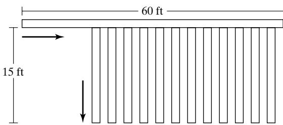 Cases enter the system from the left at a rate of 50 per minute at random times. All cases are 18 by 12 inches and travel along the 18-inch dimension. The incoming mainline conveyor is 20 inches
wide and 60 feet in length (as shown). The sortation lanes are numbered 1 to 12 from left to right, and are 18 inches wide and 15 feet in length, with 2 feet of spacing between adjacent lanes. (Estimate any other dimensions that are needed.) The infeed conveyor runs at 180 feet/minute, the sortation lanes at 90 feet/minute. All conveyor sections are accumulating, but, upon entrance at the left, incoming cases are at least 2 feet apart from leading edge to leading edge. On the sortation lanes, the cases accumulate with no gap between them.
Incoming cases are distributed to the 12 lanes in the following proportions:
| 1 | 6% | 7 | 11% |
|---|---|---|---|
| 2 | 6% | 8 | 6% |
| 3 | 5% | 9 | 5% |
| 4 | 24% | 10 | 5% |
| 5 | 15% | 11 | 3% |
| 6 | 14% | 12 | 0% |
The 12th lane is an overflow lane; it is used only if one of the other lanes fill and a divert is not possible.
At the end of the sortation lanes, there is a group of operators who scan each case with a barcode scanner, apply a label, and then place it on a pallet. Operators move from lane to lane as necessary to avoid allowing a lane to fill. There is one pallet per lane, each holding 40 cases. When a pallet is full, assume a new empty one is immediately available. If a lane fills to 10 cases and another case arrives at the divert point, this last case continues to move down the 60-foo mainline conveyor and is diverted into lane 12, the overflow lane.
Assume that one operator can handle 8.5 cases per minute, on the average. Ignore walking time and assignment of an operator to a particular lane; in other words, assume the operators work as a group uniformly spread over all 12 lanes.
(a) Set up an experiment that varies the number of operators and addresses the question: How many operators are needed? The objective is to have the minimum number of operators bu also to avoid overflow.
(b) For each experiment in part (a), report the following output statistics:
operator utilization;
total number of cases palletized;
number of cases palletized by lane;
number of cases to the overflow lane.
(c) For each experiment in part (a), verify that all cases are being palletized. In other words, verify that the system can handle 50 cases per minute, or explain why it cannot.
- Redo Exercise 1 to a greater level of detail by modeling operator walking time and operator assignment to lanes. Assume that operators walk at 200 feet per minute and that the walking distance from one lane to the next is 5 feet. Handling time per case is now assumed to be 7.5 cases per minute. Devise a set of rules that can be used by operators for lane changing. (Hint: For example, change lanes to that lane with the greatest number of cases only when the current lane is empty or the other lane reaches a certain level.) Assume that each operator is assigned to a certain number of adjacent lanes and handles only those lanes. However, if necessary, two operators (but no more) may be assigned to one lane; that is, operator assignments may overlap.
(a) If your lane-changing rule has any numeric parameters, experiment to find the best settings. Under these circumstances, how many operators are needed? What is the average operator utilization?
(b) Does a model that has more detail, as does Exercise 2(a) when compared to Exercise 1, always have greater accuracy? How about this particular model? Compare the results of Exercise 2(a) to the results for Exercise 1. Are the same or different conclusions drawn?
(c) Devise a second lane-changing rule. Compare results between the two rules. Compare tota walking time or percent of time spent walking between the two rules.
Suggestion: A lane-changing rule could have one or two “triggers.” A one-trigger rule might state that, if a lane reached a certain level, the operator moved to that lane. (Hint: Withou modification, such a rule could lead to excessive operator movement, if two lanes had about the same number of cases near the trigger level.) A two-trigger rule might state that, if a lane reached a certain level and the operator’s current lane became empty, then change to the new lane; but if a lane reaches a specified higher critical level, then the operator immediately changes lanes.
(d) Compare your results with those of other students who may have used a different lanechanging rule.
Redo Exercise 2 with a different operator-assignment rule. Basically, operators can be assigned to any lane as conditions warrant, but, as before, no more than two operators can be assigned to a lane at the same time. Address the same questions (a)–(d) as in Exercise 2.
A package-sortation system consists of one in-feed conveyor, 12 sortation lanes (or chutes), and a take-away conveyor, as shown in the following schematic (not to scale):
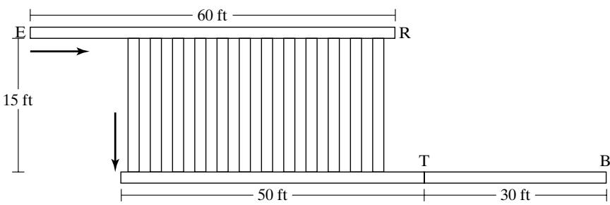
Packages enter the system from the left (at point E) at a rate of 100 per minute at random times. A package is diverted to a sortation lane on the basis of its shipping destination; in the model, a given percentage of the packages chosen randomly, according to the proportions in the nex table, are assigned to each lane. The percentages for each lane/destination is as follows:
| 1 | 6% | 7 | 10% |
|---|---|---|---|
| 2 | 6% | 8 | 6% |
| 3 | 5% | 9 | 4% |
| 4 | 24% | 10 | 4% |
| 5 | 15% | 11 | 3% |
| 6 | 14% | 12 | 3% |
After a slug of 8 packages has accumulated, they are all released together onto a 50-foot section of takeaway conveyor and head toward the point labeled T; they transfer there (at conveyor speed) onto a second section of takeaway conveyor at the end of which is a bar-code scanner (at the point labeled B). A slug cannot be released until the previous slug has cleared the point T. In this model, packages disappear at point B.
All packages are 18 by 12 inches and travel along their 18-inch dimension. The incoming mainline conveyor is 20 inches wide and 60 feet in length (as shown). The 12 sortation lanes are 18 inches wide and 15 feet in length with 2 feet of spacing between adjacent lanes. (Estimate any other dimensions that are needed.) The infeed conveyor runs at 240 feet/minute, the sortation lanes at 90 feet/minute. The infeed and sortation conveyor sections are accumulating, but, upon entrance at the left, incoming packages are at least 2 feet apart from leading edge to leading edge. On the sortation lanes, the packages accumulate with no gap between them. The 50-foo section of takeaway conveyor is a nonaccumulating belt-type conveyor; the 30-foot section is accumulating.
When a lane contains 8 packages, no more diverts are allowed until the lane is released and the slug completely clears the bottom of the chute. When a lane is full or before the slug has cleared, if another package arrives to divert, the affected package does not divert, but rather moves to the end of the infeed conveyor and then recirculates to the start of the infeed conveyor on a conveyor that is not shown in the schematic. Simulate recirculation as a time delay of 45 seconds withou explicitly modeling the recirculation conveyor itself.
(a) Set up an experiment to discover the minimum speed required of the takeaway conveyor to minimize or eliminate recirculation. Conveyors available from vendors have speeds starting at 60 feet/minute and increasing in increments of 30 feet/minute. (Faster conveyor is more expensive, so minimizing the speed will reduce costs, provided that recirculation is not a problem.)
(b) Could destination assignment to available lane be modified in such a way as to improve system performance? Devise a better assignment rule and test it, using the simulation model.
- A fleet of AGVs (Automated Guided Vehicles) services 5 workstations in series by transporting parts on fixtures from one workstation to the next, remaining with a part from the pickup point through all workstations to the offload point. The incoming staging conveyor, theAGV guidepath, the five workstations (A–E), and the offload conveyor are shown in the following schematic (not to scale):
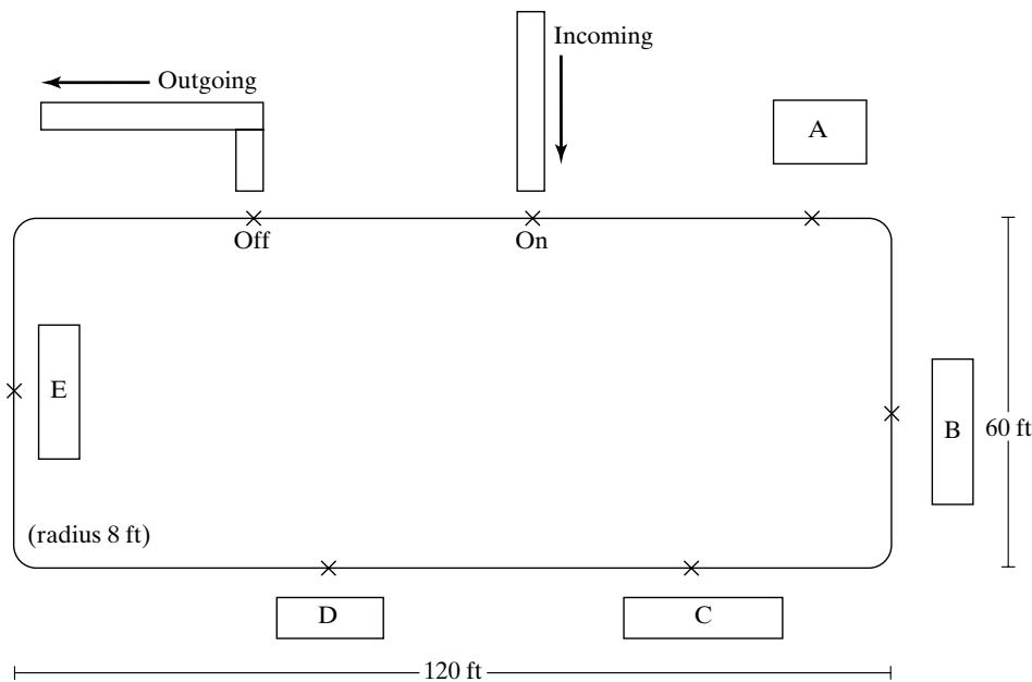
AGVs travel in a clockwise direction. Initially, all are empty and queued at the incoming conveyor at the “On” point. The workstations are labeled A–E. Parts on fixtures are staged on the incoming conveyor and picked up by an AGV at the point labeled “On”. The AGV then travels to machine A and stops at the point marked on the guidepath. The part and fixture remain on the AGV during processing, then travel together to the next workstation. After processing is completed at workstation E, the AGV travels to the point labeled “Off” the part with fixture is automatically unloaded onto the offload conveyor, and the empty AGV queues at the point labeled “On” for the next part.
Assume that the incoming conveyor remains full. It is 15 feet long and can hold 3 parts with fixtures, each taking 5 feet of conveyor space. Therefore, when one part with fixture is picked up by an AGV, another part and fixture are placed on the end of the conveyor. Pickup time is 30 seconds. The incoming conveyor runs at 30 feet per minute.
When a part has completed processing at all workstations and has been transported to the offload point labeled “Off” the offload operation takes 45 seconds. The offload conveyor itself runs at 30 feet per minute. The parts and fixtures, although taking up a space of 3 feet by 3 feet, require 5 feet on the conveyor.
Initial workstation placements are shown in approximate fashion, with no exact locations given. Constraints are that each workstation must be placed along the straight section of guidepath on which they are shown on the schematic, with the AGV stopping point no closer than 5 feet from the entrance to or exit from a curve. The incoming and offload conveyor must be placed as shown, with the offload point 20 feet from the end of the preceding curve and the pickup poin 40 additional feet to the right. Otherwise, AGV stopping points at workstations can be placed at any desired location on the straight section of guidepath.
AGVs travel at 15 feet per second and accelerate and decelerate at 3 ft/sec/sec. They are 7 feet in length and queue 8 feet apart (1 foot gap between two AGVs) when waiting for the processing position at a workstation and when in the pickup/offload position at a conveyor.
At each of the workstations, processing-time-per-part, mean-time-to-failure (MTTF), and meantime-to-repair (MTTR) are as follows:
| Workstation | Processing Time (sec.) | MTTF (min.) | MTTR (min.) |
|---|---|---|---|
| A | 120 | 90 | 3.1 |
| B | 100 | 82 | 4.0 |
| C | 140 | 110 | 4.5 |
| D | 45 | 20 | 5.0 |
| E | 100 | 240 | 9.0 |
Detailed data is not available, so certain assumptions regarding time to failure and time to repair are made: Assume that actual time to failure is exponentially distributed, with the specified mean (MTTF). Assume that repair time requires a maintenance person and that there is only one available. Actual repair times are uniformly distributed, with the mean as shown and a halfwidth of one-half the mean. Time to failure is measured against wall-clock time, not agains station-busy time. After a repair, any remaining processing time is taken, and the part continues.
There are three basic questions:
(1) What is maximum system throughput?
(2) How many AGVs are needed?
(3) What is the best workstation placement (within the stated constraints)?
For each set of experiments in parts (a) and (b), consider the following issues:
(1) Should there be a warmup period for loading the system during which no statistics are collected?
(2) How long should the simulation run?
(One suggestion: The warmup period should last at least until several parts have completed processing. The run length should allow for at least 10 downtimes on each machine. Simulate with as many AGVs as will reasonably fit on the guidepath and then try to reduce the number without reducing throughput.)
Your experiments should vary the number of AGVs and the workstation placement. Before simulating, make your best estimate regarding workstation placement, and justify that choice. Also, make a reasonable estimate regarding the likely range for number of AGVs.
(a) In the first set of experiments, use a rough-cut model that does not model theAGVs explicitly. Compute the approximate travel time between adjacent workstations and use this value as a time delay in the model. Assume there are sufficient AGVs. (Hint: Use this model to address the question of maximum throughput, but not the number of AGVs needed.) What are the advantages and limitations of this approach?
(b) In the second set of experiments, model the AGVs and guidepath explicitly. Design an experiment to find out the maximum system throughput (in parts per hour) with the smallest number of AGVs.
- More accurate information has been obtained on failure times for the workstations in Exercise 5. Redo Exercise 5 with the new information. Failures appear to be related more closely to the number of parts processed than to the amount of time passed. The new data is as follows:
| Workstation | MTTF (parts) | MTTR (min.) |
|---|---|---|
| A | 45 | 3.1 |
| B | 49 | 4.0 |
| C | 47 | 4.5 |
| D | 27 | 5.0 |
| E | 144 | 9.0 |
Note that MTTF (mean-time-to-failure) is measured in terms of number of parts, but assumptions about time to repair are unchanged from Exercise 5. For example, for Workstation A, if time to failure happened to be 45 parts, then after a failure, the 45th part would experience the next failure. In reality, failure occurs during processing, but for modeling purposes, assume the failure occurs just as processing begins. (Does this make any difference?)
For the distribution of time to failure, assume a discrete uniform distribution with mean (MTTF) over the range from 1 to 2*MTTF 1. For example, for Workstation A, the actual times to failure are equally likely to be any value from 1 to 89 parts.
Address the same questions as in Exercise 5. Do these new assumptions make any difference? How many failures are there per 8-hour shift for the first set of assumptions as compared with those for the revised assumptions?
- For the problem in Exercises 5 and 6, a study was done to evaluate the repair times more accurately for each workstation. It was found that a triangular distribution provided a closer fi
to the actual repair times. Assume the following parameters for the triangular distribution:
| Workstation | Repair Time (Triangular Distribution) | |||
|---|---|---|---|---|
| Minimum(min.) | Most Likely(min.) | Maximum(min.) | Average(min.) | |
| A | 1.0 | 2.3 | 6.0 | 3.1 |
| B | 2.0 | 3.0 | 7.0 | 4.0 |
| C | 2.5 | 3.5 | 7.5 | 4.5 |
| D | 2.0 | 4.0 | 9.0 | 5.0 |
| E | 4.0 | 7.0 | 16.0 | 9.0 |
Note that the average repair times are identical to the assumed averages (MTTR) in Exercises 5 and 6, but the distribution is triangular instead of uniform. (Most simulation languages or simulators have a built-in triangular distribution that requires specification ofthe minimum value, most likely value or mode, and maximum value. The average value is given for informational purposes only; it is the sum of the other three parameters divided by 3.)
(a) Redo Exercise 5, but with the new assumptions for repair times.
(b) Redo Exercise 6, but with the new assumptions for repair times.
- One approach to modeling downtimes discussed in this chapter, but not recommended, was to replace the processing time with a larger adjusted processing time and to leave out the downtimes. The adjusted processing time is meant to account for downtimes, at least in the long run and on the average. How would this method have affected the results for Exercise 5?
(a) For Exercise 5, compute the adjusted processing times for each workstation.
(b) For Exercise 5, use the adjusted processing times and leave out all explicit downtimes due to failure. How does this change the results? Is this a good approach for this model?
Suppose that improved maintenance and better machines could totally eliminate downtime due to failure for the system in Exercise 5. By how much would throughput improve?
Develop a model for Example 1 and attempt to reproduce qualitatively the results found in the text regarding different assumptions for simulating downtimes. Do not attempt to get exactly the same numerical results, but rather to show the same qualitative results.
(a) Do your models support the conclusions discussed in the text? Provide a discussion and conclusions.
(b) Make a plot of the number of entities in the queue versus time. Can you tell when failures occurred? After a repair, about how long does it take for the queue to get back to normal?
- In Example 1, the failures occurred at low frequency compared with the processing time of an entity. Time to failure was 1000 minutes, and interarrival time was 10 minutes, implying that few entities would experience a failure. But, when an entity did experience a failure (of 50 minutes, on average), it was several times longer than the processing time of 7.5 minutes.
Redo the model for Example 1, assuming high-frequency failures. Specifically, assume that the time to failure is exponentially distributed, with mean 2 minutes, and the time to repair is exponentially distributed, with mean 0.1 minute or 6 seconds. As compared with the lowfrequency case, entities will tend to experience a number of short downtimes.
For low-frequency versus high-frequency downtimes, compare the average number of downtimes experienced per entity, the average duration of downtime experienced, the average time to complete service (including downtime, if any), and the percent of time down.
Note that the percentage of time the machine is down for repair should be the same in both cases:
Verify percentage downtime from the simulation results. Are the results identical? . . . close? Should they be identical, or just close? As the simulation run length increases, what should happen to the percentage of time down?
With high-frequency failures, do you come to the same conclusions as were drawn in the text regarding the different ways to simulate downtimes? Make recommendations regarding how to model low-frequency versus high-frequency failures.
Redo Exercise 11 (based on Example 1), but with one change: When an entity experiences a downtime, it must be reprocessed from the beginning. If service time is random, take a new draw from the assumed distribution. If service time is constant, it starts over again. How does this assumption affect the results?
Redo Exercise 11 (based on Example 1), but with one change: When an entity experiences a downtime, it is scrapped. How does scrapping entities on failure affect the results in both the low-frequency and in the high-frequency situations? What are your recommendations regarding the handling of low- versus high-frequency downtimes when parts are scrapped?
Sheets of metal pass sequentially through 4 presses: shear, punch, form, and bend. Each machine is subject to downtime and die change. The parameters for each machine are as follows:
| Press | Process Rate (per min.) | Time to Failure (min.) | Time to Repair (min.) | No. of Sheets to a Die Change (no. sheets) | Time to Change Die (min.) |
|---|---|---|---|---|---|
| Shear | 4.5 | 100 | 8 | 500 | 25 |
| Punch | 5.5 | 90 | 10 | 400 | 25 |
| Form | 3.8 | 180 | 9 | 750 | 25 |
| Bend | 3.2 | 240 | 20 | 600 | 25 |
Note that processing time is given as a rate; for example, the shear press works at a rate of 4.5 sheets per minute. Assume that processing time is constant. The automated equipment makes the time to change a die fairly constant, so it is assumed to be always 25 minutes. Die changes occur between stamping of two sheets after the number shown in the table have gone through a machine. Time to failure is assumed to be exponentially distributed, with the mean given in the table. Time to repair is assumed to be uniformly distributed, with the mean taken from the table and a half-width of 5 minutes. When a failure occurs, 20% of the sheets are scrapped. The remaining 80% are reprocessed at the failed machine after the repair.
Assume that an unlimited supply of material is available in front of the shear press, which processes one sheet after the next as long as there is space available between itself and the next machine, the punch press. In general, one machine processes one sheet after another continuously, stopping only for a downtime, for a die change, or because the available buffer space between itself and the next machine becomes full. Assume that sheets are taken away after bending at the bend press. Buffer space is divided into 3 separate areas, one between the shear and the punch presses, the second between the punch and form presses, and the last between form and bend.
(a) Assume that there is an unlimited amount of space between machines. Run the simulation for 480 hours (about 1 month with 24-hour days, 5 days per week). Where do backups occur? If the total buffer space for all three buffers is limited to 15 sheets (not counting before shear or after bend), how would you recommend dividing this space among the three adjacent pairs of machines? Does this simulation provide enough information to make a reasonable decision?
(b) Modify the model so that there is a finite buffer between adjacent machines. When the buffer becomes full and the machine feeding the buffer completes a sheet, the sheet is not able to exit the machine. It remains in the machine, blocking additional work. Assume that tota buffer space is 15 sheets for the 3 buffers.
Use the recommendation from part (a) as a starting point for each buffer size.Attempt to minimize the number of runs. You are allowed to experiment with a maximum of 3 buffer sizes for each buffer. (How many runs does this make?) Run a set of experiments to determine the allocation of buffer space that maximizes production. Simulate each alternative for at least 1000 hours.
Report total production per hour on the average, press utilization (broken down by percentage of time busy, down, changing dies, and idle), and average number of sheets in each buffer.